
Simulate Missingness Mechanisms and Compare Analysis Results
Here is the uncomfortable truth about missing data: in a real dataset, you never see the values that went missing. You cannot check whether your imputation…

Key topics
Here is the uncomfortable truth about missing data: in a real dataset, you never see the values that went missing. You cannot check whether your imputation was right, because the answer key was deleted along with the data.
A simulation flips that. You generate the complete data first, keep a copy, then delete values yourself under a rule you control. Now you hold the answer key. Missing-data handling stops being a matter of faith and becomes an experiment you can run and score.
This tutorial builds that experiment. We will create two missingness scenarios — one purely random, one driven by an observed column — then compare complete-case analysis and simple imputation against the truth we already know.
Why Simulate Missingness at All
You already know from working with tabular data that an imputed value is an estimate, not a fact, and that imputation must be fit on training data only to avoid leakage. Those are decisions. This article is about measurement.
The payoff of simulation is a measurable gap: the distance between what your analysis reports and what is actually true. In real data that gap is invisible. In a simulation you can compute it directly, per mechanism, per strategy, per missing rate.
Think of it as a diagnostic lab, not a production pipeline. We are not choosing a strategy here. We are building a harness that scores any strategy you hand it.
The Three Mechanisms in Plain Language
The mechanism is a property of the deletion rule, not of the resulting table. That distinction matters more than any formula.
- MCAR (missing completely at random): the coin flip ignores every column, observed or not. A lab sample is dropped and breaks. Nothing about the data predicts it.
- MAR (missing at random, covariate-dependent): the coin is weighted by something you can see — another column in the table. Older patients skip a survey question more often, and age is recorded.
- MNAR (missing not at random): the coin is weighted by the value that is about to disappear. People with the highest incomes decline to report income.
Formally, the probability of missingness depends on nothing (MCAR), on observed data (MAR), or on the missing value itself (MNAR). That is enough notation. The rest is code.
We will simulate MCAR and covariate-dependent missingness. MNAR is harder to simulate honestly because you must assume a rule for values you cannot see — we will treat it as a boundary, not a target.
Knowledge check
Check your understanding
Answer this question before you continue.
Build the Complete Dataset First
You need NumPy, pandas, and scikit-learn. Fix a random seed so every run is reproducible.
import numpy as np
import pandas as pd
from sklearn.linear_model import LinearRegression

rng = np.random.default_rng(42)
n = 400

age = rng.normal(45, 12, n)
income = 30 + 0.8 * age + rng.normal(0, 8, n)
score = 5 + 0.3 * age + 0.6 * income + rng.normal(0, 5, n)

df = pd.DataFrame({"age": age, "income": income, "score": score})
The target score is built from a known formula plus noise. That formula is our ground truth. Fit a model on the complete data and record the coefficients:
def fit_coefs(frame):
    X = frame[["age", "income"]]
    y = frame["score"]
    model = LinearRegression().fit(X, y)
    return model.coef_

true_coefs = fit_coefs(df)
print("true coefficients:", true_coefs)
You should see values close to [0.3, 0.6]. That is your benchmark. Every corrupted run gets scored against it.
Knowledge check
Check your understanding
Answer this question before you continue.
Delete Values Under a Controlled Rule
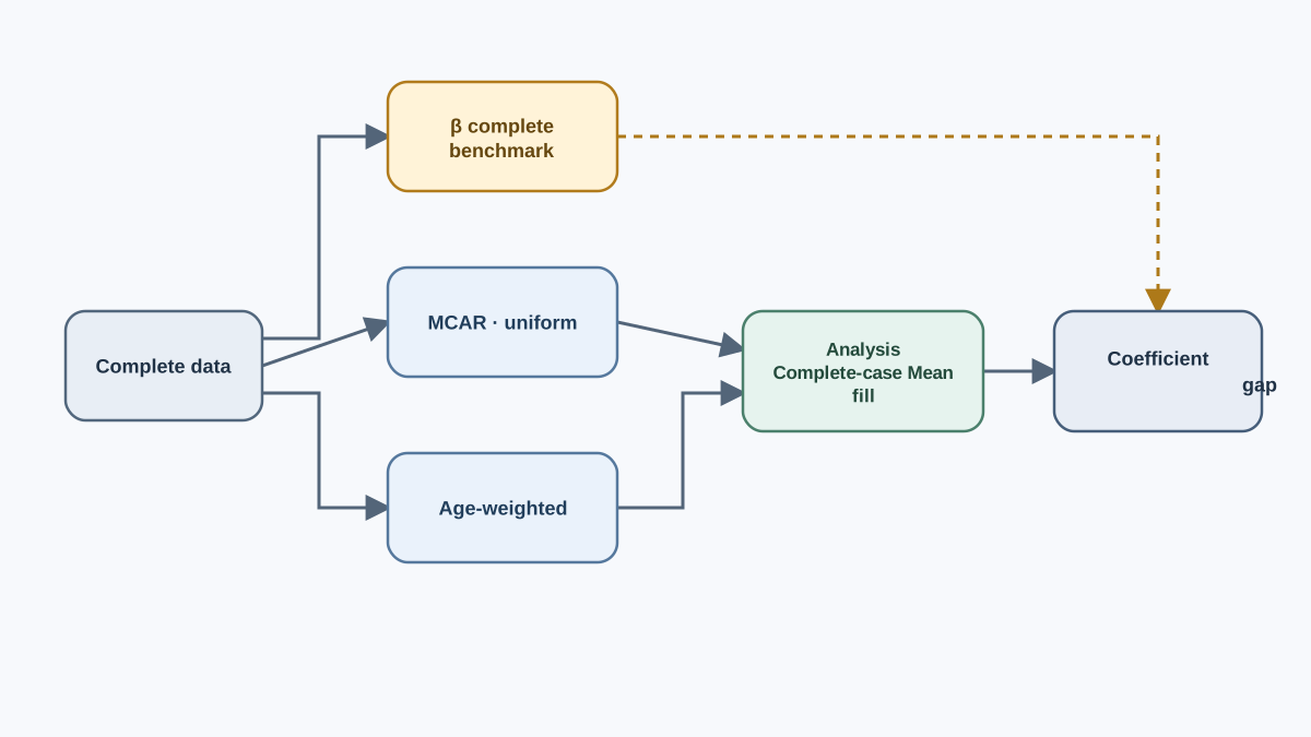
Now write the deletion rules as explicit functions. The mechanism is code you wrote — make it inspectable.
def make_mcar(frame, column, rate, rng):
    out = frame.copy()
    idx = rng.choice(out.index, size=int(rate * len(out)), replace=False)
    out.loc[idx, column] = np.nan
    return out

def make_covariate_dependent(frame, column, driver, rate, rng):
    out = frame.copy()
    # weight deletion probability by the driver column
    w = out[driver] - out[driver].min()
    p = (w / w.sum()) * rate * len(out)
    p = np.clip(p, 0, 1)
    mask = rng.random(len(out)) < p
    out.loc[mask, column] = np.nan
    return out
The first rule samples row indices uniformly. The second weights deletion by age, so older rows lose income more often.
Before trusting anything downstream, verify the mechanism actually fired:
mcar = make_mcar(df, "income", 0.3, rng)
cov  = make_covariate_dependent(df, "income", "age", 0.3, rng)

print("MCAR missing rate:", mcar["income"].isna().mean())
print("Cov missing rate:", cov["income"].isna().mean())
print("mean age, missing rows:", cov.loc[cov["income"].isna(), "age"].mean())
print("mean age, present rows:", cov.loc[cov["income"].notna(), "age"].mean())
Failure signal: A realized missing rate that differs from your target is usually just sampling variation, not a broken rule. The rate is an expected value, not a guarantee. To judge whether the mechanism is misconfigured, repeat the deletion across several seeds and check that the average rate lands near your target. Only a persistent, systematic gap points to a weighting bug.
For the covariate-dependent case, the mean age of missing rows should be visibly higher than the mean age of present rows. That difference is the mechanism, made visible.
Knowledge check
Check your understanding
Answer this question before you continue.
Compare Complete-Case and Simple Imputation Against the Truth
Two strategies, two corrupted datasets, one truth.
def complete_case(frame):
    return fit_coefs(frame.dropna())

def mean_impute(frame):
    out = frame.copy()
    out["income"] = out["income"].fillna(out["income"].mean())
    return fit_coefs(out)

for name, frame in [("MCAR", mcar), ("covariate", cov)]:
    cc = complete_case(frame)
    mi = mean_impute(frame)
    print(name, "| complete-case:", cc, "| mean-impute:", mi)
| Scenario | Strategy | Income coefficient | Gap from truth (0.6) |
|---|---|---|---|
| Complete | — | ~0.60 | 0.00 |
| MCAR | complete-case | ~0.60 | small |
| MCAR | mean impute | ~0.60 | small |
| Covariate | complete-case | shifted | larger |
| Covariate | mean impute | shifted | larger |
The pattern is the lesson. Under MCAR, both strategies land close to the truth, because the surviving rows are still a fair sample. Under covariate-dependent deletion, complete-case analysis drops the older, higher-income rows disproportionately. The remaining sample is no longer representative, and the estimate drifts.
Common mistake: Drawing conclusions from a single seed. One run is one draw, not a distribution. Repeat the simulation a few times before you believe the gap.
Knowledge check
Check your understanding
Answer this question before you continue.
What the Experiment Proves — and What It Cannot
The simulation proves the mechanism drives the distortion, because you wrote the mechanism and you hold the answer key. That is a real, defensible claim.
It does not prove anything about which mechanism produced the missing values in a dataset someone handed you. In real data, MCAR, MAR, and MNAR can produce identical-looking tables. The observed pattern does not carry the label.
This is why the honest deliverable is a sensitivity check, not a diagnosis. You can test how much your conclusion moves under different assumed mechanisms. You cannot read the mechanism off the data.
Extend the Experiment
One modification deepens the lesson and turns your script into a reusable tool: sweep the missing rate.
for rate in [0.05, 0.1, 0.2, 0.3, 0.5]:
    frame = make_covariate_dependent(df, "income", "age", rate, rng)
    gap = abs(complete_case(frame)[1] - true_coefs[1])
    print(f"rate={rate:.2f}  gap={gap:.3f}")
Watch the gap grow as the missing rate climbs. Other extensions worth trying: swap mean imputation for a model-based fill and see whether the gap shrinks under covariate-dependent deletion; loop the whole simulation over many seeds and report the spread instead of one number.
The reusable payoff is the harness itself. It scores any imputation strategy you are considering, against a truth you control.
Where This Leaves You
When you meet missing values in real data, you cannot name the mechanism. So do not pretend to. Instead, run this harness with a few assumed mechanisms, report the range of results, and let the range carry the uncertainty.
Your next step: take the same harness and point it at a model-based imputer instead of mean fill. Then wire the chosen strategy into a leakage-safe pipeline, so the imputation is fit on training data only. The lab taught you what the mechanism does. The pipeline keeps it from leaking into your evaluation.
Knowledge check
Final check
Finish the article by checking the ideas you just learned.
References
Build stronger machine learning foundations
Use structured resources to connect theory, scikit-learn workflows, and evaluation practice.


