
Derive PCA: Variance-Maximizing Directions and Covariance Eigenvectors
You can call PCA(), read explained_variance_ratio_, and get a working result. Then someone asks why the principal directions are eigenvectors of the…

Key topics
You can call PCA(), read explained_variance_ratio_, and get a working result. Then someone asks why the principal directions are eigenvectors of the covariance matrix, and the room goes quiet. This article closes that gap. We will turn "find the direction of most variance" into a constrained optimization problem, solve it, and watch the covariance matrix fall out of the algebra.
Why the Eigenvector Answer Feels Like a Trick
Most learners meet PCA in the reverse order. First they see the code, then the explained variance output, then a sentence that says the components are eigenvectors of the covariance matrix. The sentence gets memorized. It never gets derived.
That is a fragile way to know something. If you cannot reconstruct why the answer is an eigenvector, you cannot reason about what happens when you standardize your features, when you keep three components instead of two, or when a high-variance direction turns out to be useless for prediction.
So here is the plan. We define notation, write the variance objective, add the constraint that makes it solvable, and let the eigenvector equation appear as a consequence rather than an assumption. Then we extend the argument to the second component and beyond, and finish by explaining how centering and scaling change the answer — and why preserved variance is not the same as predictive relevance.
Notation and Assumptions Before Any Algebra
Let be your data matrix with rows (samples) and columns (features). Each row is one observation. Each column is one variable.
Define the centered data matrix:
where is the vector of column means and is a column of ones. Centering subtracts the mean of each feature. This is a precondition, not a stylistic choice — we will see exactly why in a moment.
The covariance matrix is:
Some texts use instead. The choice only rescales every eigenvalue by the same constant. It does not change the eigenvectors, so it does not change the directions. Pick a convention and stay consistent.
Now project a centered sample onto a unit vector . The projection score is . The variance of those scores across all samples is:
That single expression is the whole game. Everything that follows is about maximizing it.
Three assumptions are baked in. First, the structure we care about is linear — components are linear combinations of features. Second, variance is the quantity worth maximizing. Third, directions are only meaningful relative to the scaling you chose. That last one will matter a lot later.
Note: If you have not yet built intuition for what a principal component is, start with the concept article on PCA and dimensionality reduction. Here we assume you already know components are directions of variance and that projection is how you move data onto them.
The Variance Objective and Why the Constraint Is Mandatory
Write the goal plainly:
Try to solve it as stated and you hit a wall immediately. Scale by any constant . The objective becomes . Make large and the variance grows without bound. The unconstrained problem has no maximum — only a direction that runs off to infinity.
The fix is to fix the length:
This is not a technicality. It is what makes the question well-posed. The constraint says: I do not care how long the vector is, only which way it points. Direction is the free variable. Length is pinned.
Now use a Lagrange multiplier. Define:
Take the gradient with respect to and set it to zero:
Divide by two:
There it is. The eigenvector equation did not get imported from a linear algebra textbook. It fell out of the optimization. The principal directions are eigenvectors because that is what a constrained variance maximizer has to satisfy.
Knowledge check
Check your understanding
Answer this question before you continue.
From Eigenvalue Equation to Largest Eigenvalue
The equation tells us is an eigenvector, but it does not yet tell us which one. Substitute it back into the objective:
So the variance captured by a candidate direction equals its eigenvalue. To maximize variance, pick the eigenvector with the largest eigenvalue. That is the first principal component.
Because is symmetric, its eigenvectors can be chosen orthonormal — mutually perpendicular and unit length. This is not a lucky accident. It is the property that makes the next section clean.
A worked 2×2 example
Take a covariance matrix:
The eigenvalues solve :
For , solve :
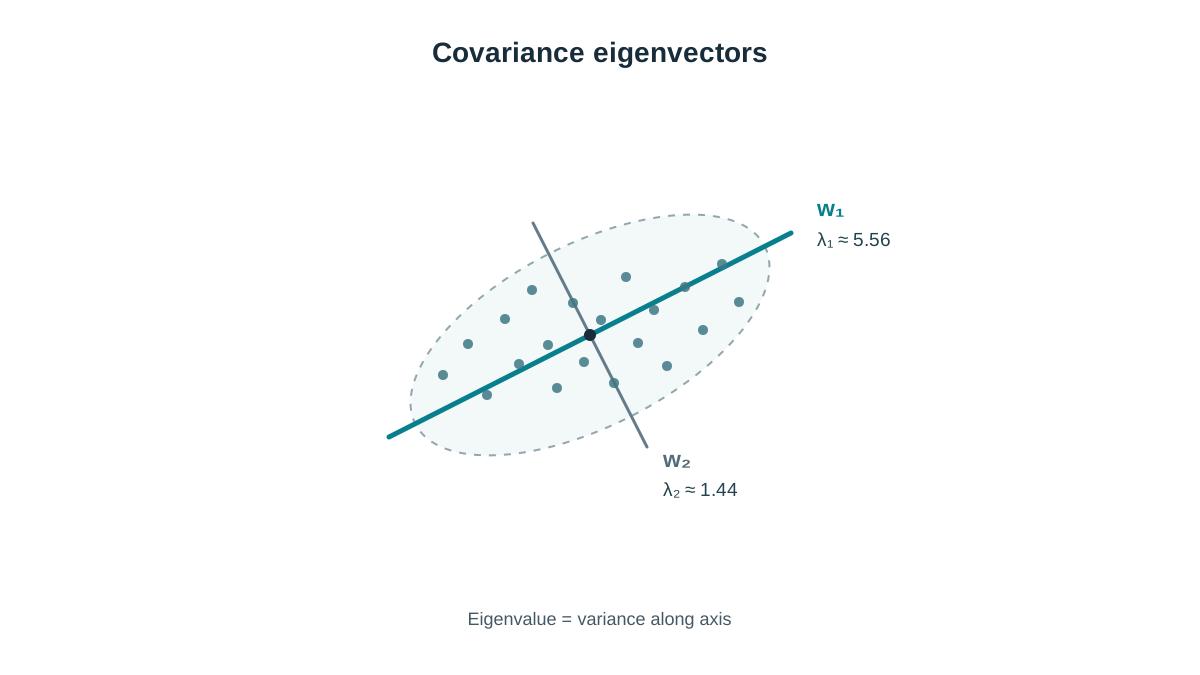
Project your centered data onto this direction and the sample variance will be approximately 5.56. Project onto the second eigenvector and you get approximately 1.44. The first direction wins because it is the eigenvector of the larger eigenvalue — exactly as the derivation predicted.
Geometrically, the leading eigenvector points along the long axis of the data cloud's ellipsoid, and the eigenvalue is that axis's squared length. The second eigenvector points along the short axis. PCA is choosing the axes of the ellipsoid that best describe the spread.
Knowledge check
Check your understanding
Answer this question before you continue.
Extending to the Second Component and Beyond
The second component faces a harder problem. It must maximize variance, stay unit length, and be orthogonal to the first component. Otherwise it would just rediscover the same direction.
Write the objective with two constraints:
The Lagrange setup now carries two multipliers:
Setting the gradient to zero gives the stationarity condition:
Now multiply both sides by from the left:
Three terms, three facts. Since is symmetric and is an eigenvector, , so . The orthogonality constraint makes . And because is unit length. Substitute all three:
The orthogonality multiplier vanishes. Drop it from the stationarity condition and you are left with — the same eigenvector equation, now restricted to the subspace orthogonal to . Maximizing within that subspace selects the eigenvector with the second-largest eigenvalue.
The pattern generalizes. The -th principal component is the eigenvector of the -th largest eigenvalue, and all components are mutually orthogonal. This is why components come out ordered by variance and why truncation keeps the top — you are keeping the directions that capture the most spread, in descending order.
The bookkeeping is clean too. The eigenvalues sum to the total variance in the data, so each explained variance ratio is just that eigenvalue's share of the sum. If and , the first component explains of the variance.
Knowledge check
Check your understanding
Answer this question before you continue.
Centering, Scaling, and How They Change the Eigenvectors
Here is where the derivation earns its keep. Two preprocessing choices change the eigenvectors themselves, not just the numbers.
Centering. The objective measures spread around the mean. If you skip centering, you are no longer eigendecomposing the covariance matrix. You are eigendecomposing the uncentered second-moment matrix, , which mixes two things: how the data varies and where the data sits relative to the origin. A feature with a large mean contributes a large diagonal entry that reflects its offset, not its spread. The leading direction can end up pointing toward the mean offset instead of the structure you care about. Centering removes that distraction, which is why ordinary PCA pipelines center first.
Scaling. Standardizing each feature to unit variance is equivalent to eigendecomposing the correlation matrix instead of the covariance matrix. The two matrices have different eigenvectors whenever features have different scales.
The consequence is concrete. Suppose one feature is measured in millimeters and another in meters. The millimeter feature has values roughly a thousand times larger, so its variance dominates the covariance matrix. The first principal component will point almost entirely at that feature — not because it carries more information, but because its units are bigger. That is a scale artifact masquerading as a finding.
Common mistake: Running PCA on unscaled features with different units and then interpreting the first component as "the most important direction." It is the most spread-out direction, which often just means the largest-unit feature.
My decision rule:
| Situation | Preprocessing |
|---|---|
| Features have different units or arbitrary scales | Standardize to unit variance |
| Features share comparable units and relative magnitude is meaningful | Keep raw covariance |
| Sparse data where centering would densify the matrix | Skip centering only if you accept the uncentered objective, or use a method built for sparse input |
That last row is a real constraint, not a loophole. Centering a sparse matrix turns zeros into nonzero means, which can blow up memory. Some pipelines avoid centering for exactly this reason, accepting a different objective in exchange for tractability. That is a deliberate trade, not a defective covariance calculation.
Knowledge check
Check your understanding
Answer this question before you continue.
What the Derivation Does Not Promise
The derivation optimizes variance. It does not optimize class separation, prediction accuracy, or causal structure. Those are different objectives, and confusing them is the most common way PCA gets misused.
A high-variance direction can be pure noise or an irrelevant nuisance variable. A low-variance direction can carry the signal you actually need. Explained variance is a property of the input representation — it says nothing about your target. A component that explains 40% of the variance in your features might explain 0% of the variation in the label you care about.
Warning: Fitting scaling or PCA on data that includes validation or test rows leaks information and inflates apparent quality. Fit on training data only, then transform the rest.
Use PCA for compression, denoising, or visualization. Validate any downstream claim with a held-out evaluation. The math guarantees preserved variance. It does not guarantee preserved usefulness.
Verify the Derivation in a Few Lines
You can confirm the theory against computation without building a full pipeline. The idea is to check that the eigenvector of the covariance matrix really does maximize projected variance.
import numpy as np

rng = np.random.default_rng(0)
X = rng.normal(size=(200, 2)) @ np.array([[2.0, 1.0], [0.0, 1.0]])

Xc = X - X.mean(axis=0)
S = Xc.T @ Xc / len(Xc)

eigvals, eigvecs = np.linalg.eigh(S)
w1 = eigvecs[:, -1]  # largest eigenvalue

projected_variance = (Xc @ w1) ** 2
print(eigvals[-1])                 # eigenvalue
print(projected_variance.mean())   # projected variance
The two printed numbers match. That is the derivation made observable: the eigenvalue is the variance along its eigenvector. Rerun the same block with standardized features — divide each column by its standard deviation — and the eigenvectors will shift, tying the code directly back to the scaling discussion.
Keep this short. The code verifies the derivation. It does not replace it.
Where This Leaves You
The eigenvectors are not a library convention. They are the solution to a constrained variance problem, and that is exactly why preprocessing choices and the variance-versus-relevance distinction matter. Once you own the derivation, scaling stops being an arbitrary rule and becomes a decision about which matrix you are eigendecomposing.
Your next step: take a real dataset, run the same verification on it, and watch how standardizing changes the leading direction. Then move to the practical PCA experiment to see these effects on real data — scaling, component count, and the gap between retained variation and predictive value.
Knowledge check
Final check
Finish the article by checking the ideas you just learned.
References
Build stronger machine learning foundations
Use structured resources to connect theory, scikit-learn workflows, and evaluation practice.


