
How Isolation Forest Turns Path Length Into an Anomaly Score
You fit an Isolation Forest, call decision_function, and get a column of numbers. You sort them, pick a cutoff, and ship the alerts. But if someone asks…

Key topics
You fit an Isolation Forest, call decision_function, and get a column of numbers. You sort them, pick a cutoff, and ship the alerts. But if someone asks why 0.62 is more anomalous than 0.55 — or why the same point scored differently after you changed max_samples — you are stuck. The score is a black box you have learned to trust.
It does not have to be. The Isolation Forest anomaly score is a normalized, inverted measure of how few random cuts it took to separate a point from everything else. Once you see that, the number stops being a confidence value the library produces and becomes a quantity you can predict, reason about, and sanity-check.
Why Short Paths Mean Unusual
Isolation Forest does not model what "normal" looks like. It does the opposite: it tries to isolate points, and it measures how much effort that took.
The mechanism is random recursive partitioning. Pick a feature at random. Pick a split value uniformly between that feature's minimum and maximum. Split the data. Recurse on each side until points are alone in their own leaf. That process builds a binary tree, and each point ends up at some leaf.
Now think about where different points land. An anomaly is few and different — it sits in a sparse region, far from the bulk of the data. A single random cut through that sparse region can carve it off. A normal point sits in a dense region where random cuts keep slicing around it, because its neighbors are everywhere. The anomaly lands near the root. The normal point lands deep.
The tree is a binary search tree in disguise. Reaching a leaf is an unsuccessful search: you followed comparisons until you fell off the end. That equivalence matters, because the average length of an unsuccessful search in a BST is a known quantity — and it will become the normalizer in the score formula.
Note: This is a geometric-density argument, not a probability model of normal behavior. The forest never learns a distribution. It only measures how quickly random axis-aligned cuts separate a point from its neighbors.
Notation: Path Length h(x) and Expected Depth E[h(x)]
Before the formula, name the pieces. Every symbol below attaches to something you just watched happen.
h(x) is the path length of point x in a single tree: the number of edges from the root to the external node where x terminates. It is the isolation depth of one point in one tree.
Leaf adjustment. When subsampling stops before every point is alone, a leaf can hold more than one point. Instead of recursing further, you add c(size) — the expected path length of the unbuilt subtree — to the edges already traversed. This keeps the depth estimate honest without growing the tree to full height.
E[h(x)] is the average of h(x) across all trees in the forest. One tree gives a noisy path; averaging over many trees turns it into a stable estimate.
n is the subsample size per tree — max_samples in scikit-learn — not the size of your full dataset. This distinction drives most misinterpretation later.
c(n) is the average path length of an unsuccessful search in a binary search tree of n nodes. It is the normalizer that makes scores comparable across different subsample sizes.
Knowledge check
Check your understanding
Answer this question before you continue.
Deriving the Score: Normalize, Then Invert
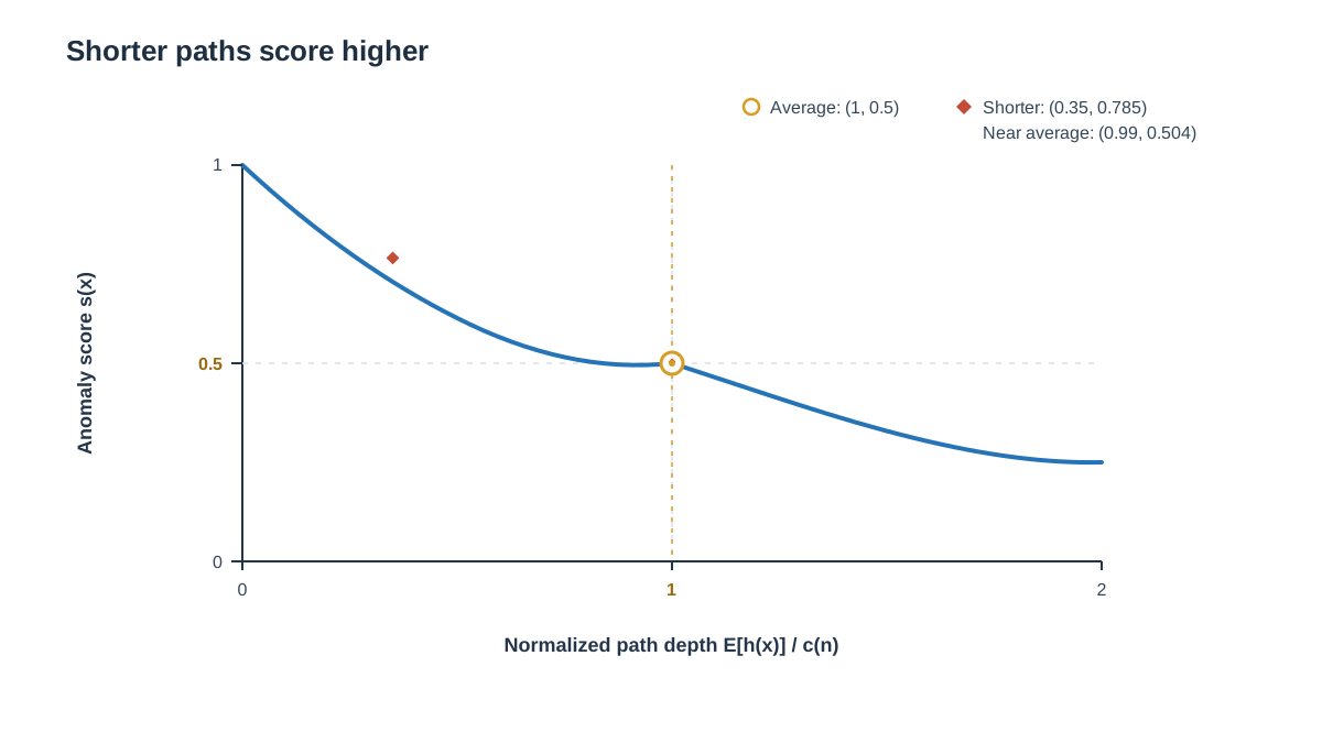
The score formula is built in two moves. Watch each one.
Step 1 — normalize. Divide E[h(x)] by c(n). Now depth is expressed as a fraction of the expected depth of a random point. A value of 1.0 means "this point took exactly as many cuts as an average point would."
Step 2 — invert. Apply:
Short paths (small depth) map to scores near 1. Long paths map to scores near 0. The inversion is what makes a high score mean anomalous.
Why the exponential instead of a simple linear flip? Two reasons. It compresses the crowded middle of the distribution and keeps the extremes readable, and it makes s = 0.5 the natural reference point: the score where depth matches the average.
The normalizer itself is:
where H(i) is the harmonic number, approximated as ln(i) + 0.5772 (the Euler–Mascheroni constant). This is the BST unsuccessful-search result. Treat it as a normalization constant, not a tunable — you do not adjust it, you inherit it from your choice of n.
Now read the anchors:
| Score | What it means |
|---|---|
| s ≈ 0.5 | Depth matches a random point — nothing unusual |
| s > 0.5 | Isolated faster than average — leaning anomalous |
| s → 1 | Isolated almost immediately — strongly isolated |
Knowledge check
Check your understanding
Answer this question before you continue.
A Worked Path-Length Example
Let's compute two scores by hand. Take n = 8, so c(n) uses H(7).
H(7) = 1 + 1/2 + 1/3 + 1/4 + 1/5 + 1/6 + 1/7 ≈ 2.5929
c(8) = 2(2.5929) − 2(7)/8 = 5.1857 − 1.75 = 3.4357
Now take two points from a forest of many trees.
Point A — a normal point sitting in a dense region. Its average depth across trees is E[h(A)] = 3.4.
s(A) = 2^(−3.4 / 3.4357) = 2^(−0.9896) ≈ 0.504
Point B — an anomaly in a sparse region. Its average depth is E[h(B)] = 1.2.
s(B) = 2^(−1.2 / 3.4357) = 2^(−0.3493) ≈ 0.785
The direction is explicit: smaller E[h(x)] produces larger s(x). The relationship is monotone decreasing. Point A lands almost exactly on the 0.5 anchor, confirming it behaves like a random point. Point B lands well above it, confirming it was isolated faster than average.
You can verify the mapping in a few lines:
import numpy as np

def c(n):
    if n <= 1:
        return 0.0
    H = np.sum(1.0 / np.arange(1, n))
    return 2 * H - 2 * (n - 1) / n

def score(expected_depth, n):
    return 2 ** (-expected_depth / c(n))

print(score(3.4, 8))  # ~0.504
print(score(1.2, 8))  # ~0.785
The Assumptions That Shape the Score
The formula is exact. What it means depends on choices you made before fitting.
Subsampling is the point, not a shortcut. Each tree sees n points, so c(n) — and therefore every score — depends on max_samples, not on dataset size. Small n works because isolation needs contrast: a small random sample preserves the "few and different" structure while keeping trees shallow and fast. But it also means your scores are relative to that sample.
Scores are relative to the training sample. The same point can score differently under a different subsample or random seed. This is not a bug; it is the nature of a randomized estimator. A point whose rank moves across seeds is a point whose isolation was sensitive to the particular sample drawn — useful information, but not a verdict on whether it is anomalous.
Feature representation can change what gets isolated. Each split picks a feature and then a value uniformly within that feature's observed range, so a positive rescaling of a single feature does not change the distribution of splits along that axis. What does change the outcome is the set of features available to cut on: adding, removing, or re-encoding features changes which directions the forest can use, and correlated or redundant features can pull splits toward directions that do not separate the anomaly. Scaling is not the lever here; feature selection and encoding are.
Axis-aligned bias. The score map is not radially symmetric. Points along feature axes can score lower than their true distance from the center suggests, because random cuts align with axes rather than following the data's shape.
What the score is not. It is not a probability. It is not calibrated across datasets. It is not a statement that a point is an error. It is a relative ranking of isolation effort.
Knowledge check
Check your understanding
Answer this question before you continue.
From Score to Decision: Thresholds and Their Limits
The 0.5 anchor is a reference point for "average depth," not a validated decision boundary. Treating it as a default cutoff is one of the most common mistakes I see.
In scikit-learn, contamination sets the threshold by assuming an anomaly rate. It encodes a prior; it does not discover one. If you set contamination=0.01, you are telling the model "assume 1% of points are anomalies" and it will return exactly that fraction.
Sign conventions will trip you up. The original paper's score s(x) increases with anomalousness. But score_samples returns the opposite of that score, and decision_function shifts it further. So "lower means more abnormal" in one call and "higher" in another. Always check which function you are reading before you sort.
The threshold itself should come from the cost of a false alert versus a missed anomaly in your actual domain — not from the shape of the score distribution. Without labels, inspect the top-ranked points against domain knowledge. Agreement is evidence, not proof.
Knowledge check
Check your understanding
Answer this question before you continue.
When This Model Fits and When It Misleads
The path-length interpretation is trustworthy when your anomalies are globally isolated — far from the bulk in at least one feature direction. It fits high-dimensional tabular data, unknown anomaly shapes, and situations where you need speed and have no labels.
It misleads when:
- Anomalies are defined by local density. A point unusual only relative to its own neighborhood will not be isolated quickly by global random cuts. Density-based methods fit better.
- Anomalies cluster. A group of similar outliers is not easy to isolate individually, because each one has neighbors.
- Features are strongly correlated. Axis-aligned cuts waste splits on redundant directions, inflating path lengths for points that are genuinely unusual in the correlated space.
The earlier decision guide on framing anomaly detection covers method selection. Here the question is narrower: does the path-length mechanism match the shape of your anomaly?
What to Do Next
Recompute your scores under two different max_samples values. Watch which points move. A point whose rank is stable across subsamples was strongly isolated — the mechanism found it regardless of the sample. A point whose rank swings is telling you that its isolation depended on the particular sample drawn; treat that as a signal to investigate further, not as proof that the point is or is not anomalous.
That instability is not a failure. It is the model telling you the truth about how much evidence it actually has. Read the Isolation Forest anomaly score as a relative ranking of isolation effort — not as a probability, not as a verdict, and not as a number that means the same thing on every dataset.
Knowledge check
Final check
Finish the article by checking the ideas you just learned.
References
Build stronger machine learning foundations
Use structured resources to connect theory, scikit-learn workflows, and evaluation practice.


