
Visualize Gradient-Descent Step Sizes on a Simple Objective
You set a learning rate, hit run, and the loss curve does something strange. Maybe it barely moves. Maybe it bounces. Maybe it turns into nan. The number…

Key topics
You set a learning rate, hit run, and the loss curve does something strange. Maybe it barely moves. Maybe it bounces. Maybe it turns into nan. The number on the screen tells you something went wrong, but not what. So let's stop guessing and run a controlled experiment where the plot itself becomes the teacher.
We will take one objective, one update rule, and several step sizes. Then we will watch each run move across the same curve and compare the trajectories side by side. By the end, you should be able to look at a loss curve and say whether it is crawling, converging, or about to blow up — and name the step-size behavior behind it.
If the basic update rule is still fuzzy, here is the one-line bridge: gradient descent moves a parameter against the gradient, scaled by the step size. The parameter update is w = w - step_size * gradient. That is the whole machine. Everything below is about what happens when you turn the step-size dial.
What We Are Testing and Why It Is Worth an Experiment
Before writing any code, let's state the question precisely, because a vague experiment teaches vague lessons.
We are testing this hypothesis: on a simple convex objective, a small step size should make slow but steady progress, a moderate step size should converge quickly, and a large step size should overshoot or diverge.
The objective is a one-variable quadratic:
f(w) = (w - 3)^2
This function has an obvious minimum at w = 3, where f(w) = 0. That is exactly why a simple objective is the right laboratory. We can compute the true answer by hand, so we are not just admiring a pretty curve — we can check whether each run actually found the minimum.
The gradient is also simple. Differentiating gives:
f'(w) = 2 * (w - 3)
Two things make this a clean experiment. First, the gradient is exact — no numerical approximation, no noise. Second, the curvature is constant, which means the stability limit is a fixed number we can reason about instead of a moving target.
Note: This is one objective with one update rule. The exact step sizes that work here do not transfer to other models. What transfers is the pattern: too small crawls, moderate converges, too large explodes.
Setup: Objective, Gradient, and Update Loop
You need Python with NumPy and Matplotlib. No scikit-learn is required — this is a from-scratch experiment, and building it by hand is the point.
Here is the smallest runnable version. The objective and its derivative are written by hand so the gradient is exact.
import numpy as np

def f(w):
    return (w - 3.0) ** 2

def grad_f(w):
    return 2.0 * (w - 3.0)

def run_gradient_descent(step_size, start=0.0, iterations=20):
    w = start
    history = {"w": [w], "loss": [f(w)]}
    for _ in range(iterations):
        w = w - step_size * grad_f(w)
        history["w"].append(w)
        history["loss"].append(f(w))
    return history
The loop records the parameter value and the loss at every iteration, not just at the end. That history is what we will plot. If you only keep the final number, you lose the entire story of how the run got there.
Let's confirm the loop runs before plotting anything:
history = run_gradient_descent(step_size=0.1)
print("iterations recorded:", len(history["w"]))
print("first few w:", [round(v, 3) for v in history["w"][:5]])
print("final w:", round(history["w"][-1], 4))
print("final loss:", round(history["loss"][-1], 6))
You should see a list of parameter values that starts at 0.0 and walks toward 3.0. The final loss should be small but not exactly zero after only 20 iterations. If your output looks like that, the loop is working and you are ready to visualize.
Knowledge check
Check your understanding
Answer this question before you continue.
Plotting Parameter and Loss Trajectories
One plot is not enough. We need two views because they answer different questions.
The parameter plot shows where the point is on the curve — direction and overshoot. The loss plot shows whether progress is monotonic — is the loss falling every step, or bouncing?
import matplotlib.pyplot as plt

def plot_run(history, step_size):
    w_vals = np.array(history["w"])
    losses = np.array(history["loss"])

    fig, (ax1, ax2) = plt.subplots(1, 2, figsize=(11, 4))

    # Left: the point hopping along the objective curve
    curve_w = np.linspace(-2, 8, 200)
    ax1.plot(curve_w, f(curve_w), color="lightgray", label="f(w)")
    ax1.plot(w_vals, losses, "o-", color="tab:blue", label="iterates")
    ax1.set_xlabel("w")
    ax1.set_ylabel("f(w)")
    ax1.set_title(f"Parameter trajectory (step={step_size})")
    ax1.legend()

    # Right: loss per iteration, log scale
    ax2.plot(losses, "o-", color="tab:red")
    ax2.set_yscale("log")
    ax2.set_xlabel("iteration")
    ax2.set_ylabel("loss (log scale)")
    ax2.set_title("Loss trajectory")

    plt.tight_layout()
    plt.show()

plot_run(run_gradient_descent(step_size=0.1), step_size=0.1)
The log scale on the loss plot matters. On a linear axis, a run that drops from 9 to 0.001 flattens into a single line near zero, and a run that diverges shoots off the top. On a log axis, slow progress and divergence are both visible on the same chart.
Here is how to read what you see:
| Pattern | Parameter plot | Loss plot |
|---|---|---|
| Monotonic descent | Points march steadily toward the minimum | Smoothly falling line |
| Flat-but-falling | Points creep, barely moving | Gentle downward slope |
| Overshoot / oscillation | Points jump past the minimum and back | Zigzag or rising line |
Knowledge check
Check your understanding
Answer this question before you continue.
Reading Three Step Sizes Side by Side
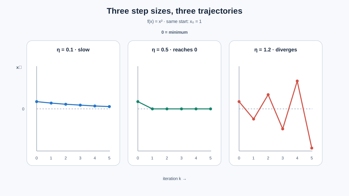
Now the actual experiment. We run the same objective with three step sizes and compare each final parameter to the known minimum at w = 3.
for step in [0.05, 0.5, 1.1]:
    h = run_gradient_descent(step_size=step, iterations=20)
    print(f"step={step:>4}  final w={h['w'][-1]:>10.4f}  "
          f"final loss={h['loss'][-1]:>12.6f}")
Small step size (0.05). The loss falls every iteration, but the parameter barely moves. After 20 iterations it is still far from 3.0. Nothing is wrong — it is just slow. Convergence would take many more iterations.
Moderate step size (0.5). The loss drops fast and the parameter settles near 3.0 within a handful of iterations. This is the run that looks "right."
Large step size (1.1). The parameter jumps past the minimum, the loss rises or oscillates, and the run never settles. This is the classic overshoot signature — the same one you will see in a real model when the learning rate is too high.
The comparison to the true minimum is what makes this a real experiment rather than a light show. You are not asking "does the curve look nice?" You are asking "did the run land near 3.0, and how many iterations did it take?"
Knowledge check
Check your understanding
Answer this question before you continue.
Why the Same Step Size Behaves Differently Here
The three behaviors are not random. They come from one relationship: step size versus curvature.
The gradient near the minimum is small, so updates are small. But far from the minimum the gradient is large, so the same step size produces a large jump. A step that is safe on a gentle curve can overshoot on a steep one. That is why the stability limit depends on the objective, not on a universal magic number.
There is a clean way to see the boundary for this specific objective. The update is w = w - step * 2 * (w - 3). The factor multiplying the distance from the minimum is (1 - 2 * step). When step is below 1.0, that factor is between -1 and 1, so the distance shrinks each iteration and the run converges. At step = 1.0 it flips sign and never shrinks. Above 1.0 it grows, and the run diverges. That is why 0.5 converges and 1.1 explodes — and it is a property of this curve, not a rule for all models.
Common mistake: Treating a learning rate that worked on one problem as a safe default for another. The safe range is tied to the objective's curvature, which changes when your data changes.
This is also why feature scaling matters in practice. Scaling changes the effective curvature of the loss surface, which moves the stability limit. Keep that as a forward pointer for now — the point here is the mechanism, not a recipe for choosing a learning rate in a real model.
Failure Modes and Debugging Signals
When your own runs go wrong, match the symptom to the cause:
- Loss flat and barely moving. Step size is likely too small, or the gradient is near zero far from the minimum.
- Loss rising or oscillating between two values. Step size is too large for this objective's curvature.
- Loss becomes
nanor infinity. The updates are diverging and the parameter is escaping to large magnitudes.
The practical debugging move is always the same: log the parameter and the loss at every iteration and plot them. A single final number cannot tell you whether the run crawled, converged, or exploded. The trajectory can.
Knowledge check
Check your understanding
Answer this question before you continue.
One Modification to Try Yourself
Change the curvature and rerun the same three step sizes. Make the quadratic steeper by editing the objective:
def f(w):
    return 5.0 * (w - 3.0) ** 2

def grad_f(w):
    return 10.0 * (w - 3.0)
Now rerun the loop with step = 0.5. On the gentler curve it converged quickly. On this steeper one it should overshoot. That single change proves the stability limit is tied to the objective, not to the number 0.5.
Before you run it, predict the outcome. Then compare your prediction to the output. The gap between the two is where the learning happens.
If you want one more variation, add a simple decaying step size — start at 0.5 and multiply it by 0.9 each iteration — and watch how it stabilizes a run that previously oscillated.
What to Carry Forward
The skill here is not memorizing three step sizes. It is reading a loss curve and naming what you see. Crawling, converging, diverging — each has a signature, and each points to a specific cause.
The numbers in this experiment belong to this objective only. But the habit does not. When you train a real model, log the loss every iteration, plot it, and inspect the shape before you touch anything else. The curve is not decoration. It is the system telling you what it is doing.
Your next step: take the same plot-and-inspect habit to a real model's training curve. Pick a small dataset, fit a simple model, and watch the loss trajectory. Then ask the same question you asked here — is this crawling, converging, or diverging?
Knowledge check
Final check
Finish the article by checking the ideas you just learned.
References
Build stronger machine learning foundations
Use structured resources to connect theory, scikit-learn workflows, and evaluation practice.


