When Gradient Descent Converges: Smoothness, Convexity, and Step Size

"Gradient descent works" and "gradient descent is guaranteed to converge" sound like the same sentence. They are not. One is a hope backed by experience. The other is a contract with named clauses, and if you cannot name the clauses, you cannot know when the contract is void.

You already know the update rule: $x_{t+1} = x_t - \eta \nabla f(x_t)$. You have watched loss curves fall and learning rates misbehave. What you have not been told is which assumptions turn that update rule into a theorem. That is what we are going to build here: a bounded convergence result you can state yourself, a step size ceiling you can derive, and a clear boundary where the guarantee stops describing your actual model.

What a Convergence Guarantee Actually Claims

A guarantee has a specific shape. It says: given assumptions A, after $t$ steps the gap $f(x_t) - f^*$ is at most some function of $t$. No assumptions, no theorem. The assumptions are the price of admission.

Three claims get blurred together in casual conversation, and they are not the same result:

• Loss decreases monotonically. Each step is no worse than the last.
• The gradient norm goes to zero. The iterates approach a stationary point.
• The iterates approach a minimizer. The parameters actually converge to $x^*$.

These need different assumptions and give different conclusions. Monotone decrease is the weakest and cheapest. Approaching a minimizer is the strongest and most expensive.

The three assumptions that do the work here are L-smoothness, convexity, and a step size bound. The rest of this article earns each one, then shows what they buy together.

Notation and the Two Assumptions That Do the Work

Fix the setting. We minimize $f: \mathbb{R}^d \to \mathbb{R}$. Write $\nabla f(x)$ for the gradient, $\eta$ for the step size, $x_t$ for the iterate after $t$ steps, $x^*$ for a minimizer, and $f^* = f(x^*)$ for the optimal value.

L-smoothness says the gradient is $L$-Lipschitz:

$\|\nabla f(x) - \nabla f(y)\| \le L\|x - y\|.$

In plain causal language: the gradient cannot change faster than $L$ per unit of movement. If you take a step, the gradient you land on is still roughly the gradient you left. That is what makes $-\nabla f(x_t)$ a usable descent direction for a while instead of a direction that goes stale mid-step.

For twice-differentiable functions there is an equivalent view that is easier to check: the Hessian eigenvalues are bounded by $L$ in magnitude, so $-LI \preceq \nabla^2 f(x) \preceq LI$. If you can bound the curvature of your objective, you have bounded $L$.

Convexity says the tangent line is a global lower bound:

$f(y) \ge f(x) + \nabla f(x)^\top (y - x).$

No misleading local valleys. Every gradient points toward a direction that genuinely improves the global objective.

Note: Smoothness is a bound on how fast curvature can change, not a promise that the function is nice in any practical sense. A function can be perfectly smooth and still have a huge $L$, which forces a tiny step size and slow progress.

The Descent Lemma: Why the Step Size Has a Ceiling

Here is where the step size bound comes from. It is not taste. It is algebra.

L-smoothness implies a quadratic upper bound on the function around any point:

$f(y) \le f(x) + \nabla f(x)^\top (y - x) + \frac{L}{2}\|y - x\|^2.$

This says: near $x$, the function sits below a parabola whose curvature is set by $L$. Substitute the gradient step $y = x - \eta \nabla f(x)$:

$f(x_{t+1}) \le f(x_t) - \eta\left(1 - \frac{L\eta}{2}\right)\|\nabla f(x_t)\|^2.$

Read the bracket. It is positive only when $\eta < 2/L$. When $\eta \le 1/L$, the bracket is at least $1/2$, so each step reduces the loss by at least $\frac{\eta}{2}\|\nabla f(x_t)\|^2$.

Two failure modes fall straight out of the inequality:

• $\eta$ too large. The bracket goes negative, the bound becomes useless, and the step can increase the loss. This is the overshoot you have seen as a diverging loss curve.
• $\eta$ very small. The bracket stays positive and safe, but each step's improvement shrinks with $\eta$. Safe and slow.

The safe ceiling scales with $1/L$. A badly scaled problem with a large $L$ forces a small step size and slow progress. That is the mechanism behind the feature-scaling advice you have already met: scaling features reduces the effective $L$ and raises the safe step size.

From Descent to a Convergence Rate

The per-step inequality bounds how much each step improves. To get a bound on the gap $f(x_t) - f^*$, we need a different potential: the squared distance from the current iterate to a minimizer.

Start by expanding that distance after one step:

$\|x_{t+1} - x^*\|^2 = \|x_t - \eta \nabla f(x_t) - x^*\|^2 = \|x_t - x^*\|^2 - 2\eta \nabla f(x_t)^\top (x_t - x^*) + \eta^2 \|\nabla f(x_t)\|^2.$

Convexity gives us the bridge we need. The tangent-line inequality, rearranged, says $\nabla f(x_t)^\top (x_t - x^*) \ge f(x_t) - f^*$. Substitute that in and drop the nonnegative $\eta^2 \|\nabla f(x_t)\|^2$ term:

$\|x_{t+1} - x^*\|^2 \le \|x_t - x^*\|^2 - 2\eta (f(x_t) - f^*).$

Rearrange to isolate the gap:

$f(x_t) - f^* \le \frac{\|x_t - x^*\|^2 - \|x_{t+1} - x^*\|^2}{2\eta}.$

Now sum both sides from $t = 0$ to $t = T - 1$. The right side telescopes — every intermediate distance cancels, leaving only the first and last:

$\sum_{t=0}^{T-1} \big(f(x_t) - f^*\big) \le \frac{\|x_0 - x^*\|^2 - \|x_T - x^*\|^2}{2\eta} \le \frac{\|x_0 - x^*\|^2}{2\eta}.$

The average gap over $T$ steps is at most $\|x_0 - x^*\|^2 / (2T\eta)$. Since the average is bounded, the best iterate is too:

$f(x_T) - f^* \le \frac{\|x_0 - x^*\|^2}{2T\eta}.$

Read the terms. A better starting point (smaller $\|x_0 - x^*\|$) helps. A larger safe step size helps. The gap shrinks like $1/T$ — sublinear. Halving the gap costs roughly twice the iterations. That is the price of weak convexity.

If you add strong convexity — a curvature floor $m$ as well as a ceiling $L$ — the same machinery gives a linear rate, $(1 - m/L)^T$. The gap shrinks by a constant factor each step. The $1/T$ rate is a consequence of weak convexity, not a universal speed limit.

Common mistake: Treating this bound as a prediction. It is a worst-case guarantee over all functions satisfying the assumptions. Real problems often converge faster. The bound says nothing about problems that violate the assumptions.

A Worked Example You Can Check by Hand

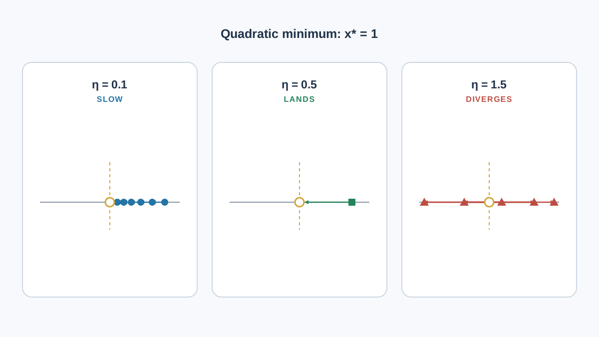
Take $f(x) = (x - 1)^2 + 10$. The second derivative is $2$, so $L = 2$ and the safe step size is $\eta = 1/L = 0.5$.

Start at $x_0 = 0$. The gradient is $\nabla f(0) = 2(0 - 1) = -2$. One step:

$x_1 = 0 - 0.5 \cdot (-2) = 1.$

The iterate lands exactly on the minimizer. The bound is tight here, not loose.

Now predict before computing. With $\eta = 0.1$, the bracket $1 - L\eta/2 = 0.9$ is positive, so the loss decreases every step — but slowly. With $\eta = 1.5$, the bracket $1 - 1.5 = -0.5$ is negative, so the descent lemma no longer guarantees anything. That is a statement about the inequality, not yet about the loss.

To see what actually happens at $\eta = 1.5$, run the update. The gradient is $2(x_t - 1)$, so:

$x_{t+1} = x_t - 1.5 \cdot 2(x_t - 1) = x_t - 3(x_t - 1) = -2x_t + 3.$

The distance from the minimizer transforms as $x_{t+1} - 1 = -2(x_t - 1)$. Each step doubles the distance and flips its sign. Starting at $x_0 = 0$, the iterates are $3, -3, 9, -21, \dots$ — oscillating with growing amplitude. The loss ratio per step is $4$, so the loss grows by a factor of four each iteration. The negative bracket told you the guarantee was gone; the update rule told you the loss diverges.

This is the smallest possible laboratory: one function, three step sizes, three visibly different behaviors. You can reproduce it in a few lines of NumPy, but the point is the prediction, not the plot.

Warning: A quadratic is the friendliest possible case. Its behavior should not be generalized to a neural network loss, where $L$ is unknown, varies across the parameter space, and convexity does not hold.

Where the Guarantee Stops Applying

The theorem is clean. Your model probably is not. Here is where the clauses break.

Non-convex losses break the convexity clause. Gradient descent can still reach a stationary point, but a stationary point is not a minimum. Worst-case guarantees for locating good minima of arbitrary non-convex functions are genuinely limited.

Stochastic gradients break the deterministic step. With minibatch noise, the loss is not guaranteed to decrease every iteration, and convergence statements become statements in expectation. This is why monitoring a validation score is often more useful than watching the training loss.

Unknown or varying $L$ breaks the fixed step size. If curvature changes across the parameter space, a single $\eta$ that is safe in one region can be too large in another. This is the motivation for adaptive and decaying step sizes.

Regularized and constrained objectives change the geometry. Adding an L2 penalty keeps convexity for many linear models but shifts the minimizer. Adding a non-convex penalty does not.

Before trusting any convergence claim, name the objective, name the assumptions it satisfies, and check whether the step size respects the bound those assumptions imply.

What to Take Into Practice

Treat the step size as a quantity with a ceiling, not a free hyperparameter. When training diverges, your first hypothesis should be that $\eta$ exceeded the local curvature, not that the model is wrong.

Scale your features before blaming the optimizer. Scaling reduces the effective $L$ and therefore raises the safe step size.

Use the assumptions as a diagnostic checklist. Smooth, convex, bounded step size — three questions to ask whenever a convergence claim sounds too strong.

Pick one objective you already use. Estimate or bound its curvature, then check whether your current step size respects $1/L$. If it does not, you now know why the loss curve looks the way it does — and you know exactly which knob to turn.