How Feature Scaling Changes Distance Geometry: A Mathematical Derivation

Two houses sit side by side in your table. One is 1,800 square feet with 3 bedrooms. The other is 2,000 square feet with 5 bedrooms. To a k-NN model, the first house is "closer" to a 1,900-square-foot, 4-bedroom house than the second one is — even though the second pair differs by the same number of bedrooms and a smaller area gap. The model is not broken. The arithmetic is doing exactly what you told it to do.

Here is the thesis I want you to carry through this article: scaling is not cosmetic normalization. It is a change of metric, and a change of metric is a change of model. Once you see the algebra, you stop treating StandardScaler as a checkbox and start treating it as a modeling decision.

If you have not yet read the intuition-level treatment of when to scale, that is the right prerequisite. This article assumes you already believe scaling matters. The question here is narrower and sharper: what exactly does scaling do to the geometry of your feature space?

The Symptom: One Column Hijacks the Distance

Take two points in two dimensions. Feature 1 is square footage, ranging from roughly 500 to 5,000. Feature 2 is bedroom count, ranging from 1 to 6.

The squared Euclidean distance between two points is the sum of squared per-feature differences:

$$d^2(x, z) = (x_1 - z_1)^2 + (x_2 - z_2)^2$$

A 1,000-square-foot difference contributes $1{,}000^2 = 1{,}000{,}000$ to that sum. A 2-bedroom difference contributes $2^2 = 4$. The area term is roughly 250,000 times larger. The bedroom signal is not "less important" in any statistical sense — it is simply outvoted by the units.

The consequence is uncomfortable: your multivariate model is effectively univariate. It picks neighbors almost entirely by square footage while pretending to use both features. The hidden question, then, is whether scaling is a cosmetic rescaling of numbers or a redefinition of the metric itself. It is the second one, and the derivation below shows exactly why.

Notation and Assumptions

Before the algebra, fix the symbols.

• A data point is a vector $x \in \mathbb{R}^d$, with coordinates indexed by $j = 1, \dots, d$.
• The difference vector between two points is $\delta = x - z$, with components $\delta_j = x_j - z_j$.
• Squared Euclidean distance is $d^2(x, z) = \sum_{j=1}^{d} \delta_j^2$.
• Because the square root is strictly increasing on nonnegative reals, ranking by $d$ and ranking by $d^2$ give the same order. We work with squares to avoid dragging the radical through every line.

Scaling is a diagonal linear map. For positive scale factors $s_1, \dots, s_d$:

$$x' = S x, \qquad S = \operatorname{diag}(s_1, \dots, s_d)$$

That is, each coordinate is multiplied by its own factor: $x'_j = s_j x_j$.

Three assumptions hold throughout the derivation. First, the scale factors are fixed positive constants — no zero, no negatives, no data-dependent randomness inside the algebra. Second, we are not yet translating; centering comes later. Third, distances are computed in the transformed space, which is the space the model actually sees. That last point matters because the scale factors are usually estimated from data, and estimated parameters are where leakage enters.

Deriving the Scaled Distance

Substitute the transformed points into the definition:

$$d^2(Sx, Sz) = \sum_{j=1}^{d} (s_j x_j - s_j z_j)^2$$

Factor $s_j$ out of each squared difference:

$$d^2(Sx, Sz) = \sum_{j=1}^{d} s_j^2 (x_j - z_j)^2 = \sum_{j=1}^{d} s_j^2 \delta_j^2$$

Define $w_j = s_j^2$. Then:

$$d^2(Sx, Sz) = \sum_{j=1}^{d} w_j \delta_j^2$$

That is the whole derivation, and it is worth pausing on. Coordinate-wise scaling turns Euclidean distance into a weighted Euclidean distance. Each original squared difference is multiplied by its own nonnegative weight. Scaling does not merely shrink numbers; it assigns importance.

Two consequences fall out immediately. The derivation holds for any positive $s_j$, including $s_j < 1$ — shrinking a dimension's influence is the same operation as amplifying another's, just with a different sign in the exponent. And the weights are squared: halving a scale factor quarters that dimension's contribution.

A Worked Example

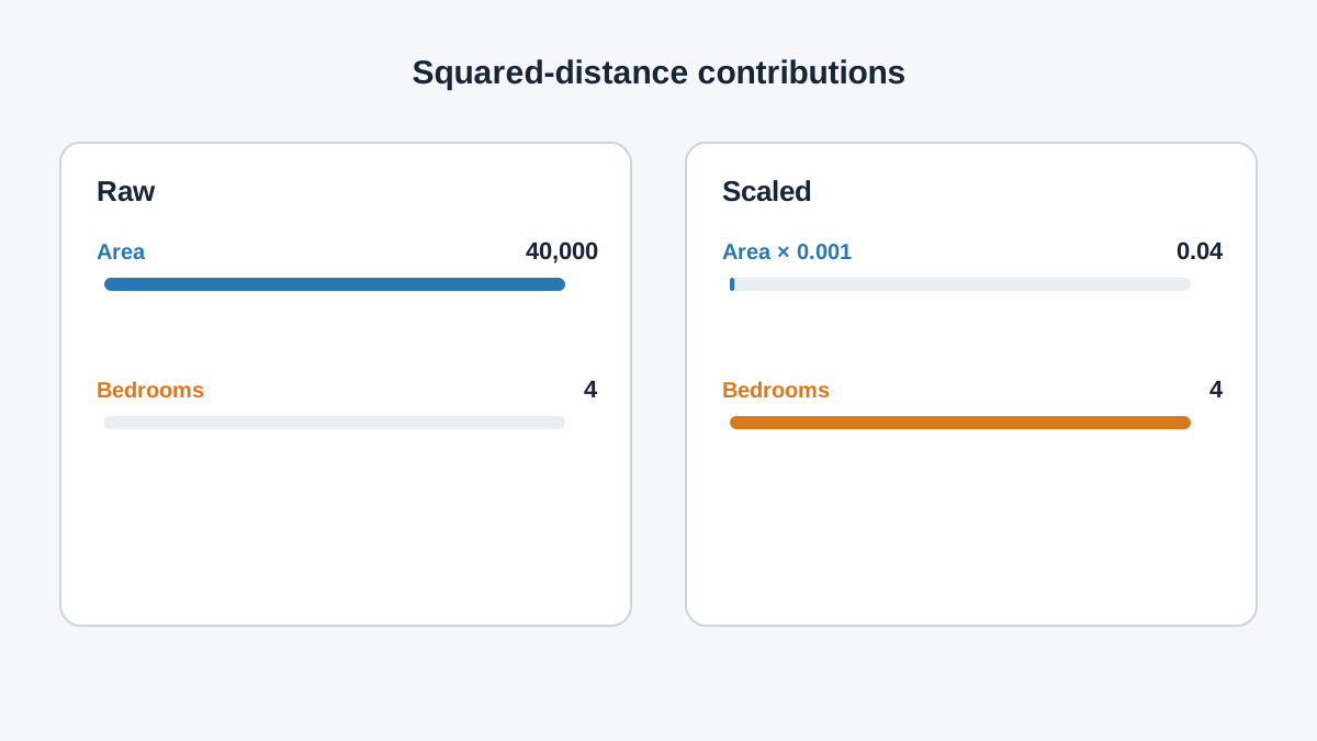
Take two points in two features: $x = (2000, 5)$ and $z = (1800, 3)$. Raw squared distance:

$$d^2 = (2000 - 1800)^2 + (5 - 3)^2 = 40{,}000 + 4 = 40{,}004$$

Now scale feature 1 by $s_1 = 0.001$ (converting square feet to thousands) and feature 2 by $s_2 = 1$ (leaving bedrooms alone). The weights are $w_1 = 10^{-6}$ and $w_2 = 1$:

$$d^2(Sx, Sz) = 10^{-6} \cdot 40{,}000 + 1 \cdot 4 = 0.04 + 4 = 4.04$$

The bedroom difference now dominates. Same two points, same table, different geometry. That is the mechanism behind every "scale your features" rule of thumb you have ever read.

δ = (4, 3)
s = (0.5, 2)

Which Transformations Preserve Neighbor Rankings

Not every transformation changes the geometry. Some leave it intact, and knowing which is which keeps you from scaling things that do not need it.

Uniform scaling. If every $s_j = c$ for a single positive constant $c$, then:

$$d^2(Sx, Sz) = \sum_j c^2 \delta_j^2 = c^2 d^2(x, z)$$

Every pairwise distance is multiplied by the same factor $c^2$. Rankings are preserved, nearest neighbors are preserved, and k-NN decisions are unchanged. Multiplying every column by the same constant is a no-op for distance-based models.

Translation. Subtracting a per-feature constant leaves every $\delta_j$ unchanged, so distances are unchanged. This is why centering is harmless — and why the mean subtraction inside standardization is not the part that matters. The division by standard deviation is.

Rotation and reflection. A square orthogonal transformation — a rotation or reflection that keeps the same number of dimensions — preserves Euclidean distances exactly. This is the geometric fact behind PCA when you retain all components: the principal axes are just a rotated coordinate system, and distances between points are unchanged. Projecting onto fewer components is a different operation. It discards directions, and discarded directions generally do not preserve all pairwise distances.

Nonuniform scaling. When the $s_j$ differ across dimensions, the ordering of distances can change. Neighbor sets change. Cluster assignments change. This is the case that matters in practice, and it is the case where the choice of scaler becomes a modeling decision.

Note: Ranking preservation is a statement about the metric, not about the model. A model that also uses a threshold, a margin, or a regularization penalty can still change behavior under uniform scaling, because those components do not live inside the distance.

Why Standardization and Min-Max Scaling Are Not the Same Geometry

The general weight formula $w_j = s_j^2$ lets us read off what each common scaler actually does.

Transformation	Scale factor $s_j$	Implied weight $w_j$	What it measures
Standardization	$1 / \sigma_j$	$1 / \sigma_j^2$	Standard-deviation units
Min-max scaling	$1 / (\max_j - \min_j)$	$1 / \text{range}_j^2$	Range units
Robust scaling	$1 / \text{IQR}_j$	$1 / \text{IQR}_j^2$	Interquartile-range units

Standardization down-weights high-variance dimensions. Min-max scaling down-weights wide-range dimensions — and a single extreme value inflates the range, shrinking that dimension's influence for every point in the dataset. Robust scaling substitutes the interquartile range, changing the weight again and reducing sensitivity to extremes.

The practical consequence: the two methods produce different weight vectors, so they can produce different neighbor sets on the same data. This is not a formatting choice. It is a choice about what the model is allowed to care about. The mechanics of each scaler belong to the prerequisite article; here, the point is that they imply different geometries.

From Weights to Decisions: What Actually Changes

The algebra predicts observable behavior. Here is what to watch for.

k-NN. Neighbor sets and predictions can flip under nonuniform scaling. If your model's accuracy jumps from mediocre to strong after scaling, the model was not learning a multivariate pattern before — it was learning a univariate one.

k-means. Cluster boundaries shift because assignment depends on distance to centroids. The objective is implicitly weighted by whatever scale factors you chose, whether you thought about it or not.

SVM with an RBF kernel. The kernel is a function of squared distance, so scaling changes the effective bandwidth per dimension and therefore the decision boundary.

Two failure modes deserve naming. First, scaling a feature that carries no signal amplifies noise into a full-weight dimension — scaling can make a model worse, not just different. Second, fitting the scaler on the full dataset before splitting leaks test-set statistics into the weights. The scale factors are parameters learned from data, and learned parameters belong on the training side of the boundary.

Common mistake: Treating the scaler as a formatting step that happens "before modeling." It is part of the model. Fit it on training data, apply it to everything else.

When Scaling Is the Wrong Move

The derivation does not imply that you should always scale. It implies that scaling is a metric choice, and some models do not use the metric you are changing.

Tree-based models split on coordinate thresholds. Monotone per-feature rescaling does not change the set of achievable splits, so scaling is usually unnecessary there. Binary and one-hot indicator features are already on a comparable 0/1 scale; rescaling them can distort the intended equal weighting. When the raw units are the meaningful signal — physical measurements, prices, durations — normalizing away the magnitude can remove information the model should use. And when outliers are the phenomenon of interest, a scaler that compresses them may hide the very structure you are trying to detect.

Verifying the Derivation in Code

Theory tells you why. Output tells you whether you understood it. Here is a compact experiment that confirms the algebra numerically.

import numpy as np

rng = np.random.default_rng(0)
X = rng.normal(size=(6, 2)) * np.array([1000.0, 3.0])

def sq_dists(A):
    diff = A[:, None, :] - A[None, :, :]
    return (diff ** 2).sum(axis=-1)

s = np.array([0.001, 1.0])
X_scaled = X * s

D_raw = sq_dists(X)
D_scaled = sq_dists(X_scaled)

# Predicted: d^2(Sx, Sz) == sum_j s_j^2 * (x_j - z_j)^2
diff = X[:, None, :] - X[None, :, :]
predicted = (diff ** 2 * (s ** 2)).sum(axis=-1)

print(np.allclose(D_scaled, predicted))   # True

# Nearest neighbor of point 0, before and after
print(np.argsort(D_raw[0])[1], np.argsort(D_scaled[0])[1])

Run it. If the nearest-neighbor index changes between the two prints, you have just watched nonuniform scaling reorder the geometry. If you set s = np.array([2.0, 2.0]) instead, every distance is multiplied by 4 and the neighbor list is identical — uniform scaling in action.

The Decision Rule

Scaling is a choice of metric, and choosing a metric is choosing what the model is allowed to care about. The derivation gives you a decision rule: pick scale factors that reflect the units and reliability you believe in, and treat that choice as part of the model specification — not as a preprocessing afterthought.

The next practical step is placing the scaler inside a leakage-safe pipeline so the weights are learned from training data only. That is where the algebra meets the workflow, and it is the difference between a model that generalizes and one that quietly memorized its test set. The same weight reasoning also explains why distance-based and kernel-based models respond to scaling while trees shrug it off: trees never asked about the metric in the first place.