Estimate a Statistic’s Uncertainty With a Reproducible Bootstrap Experiment

You have one sample, one number, and no honest way to say how much that number would move if you collected the data again. The bootstrap does not create new information. It re-asks the same question many times against the only population you actually have: your sample. Run the experiment below with a fixed seed, and you will watch a sampling distribution appear on your screen instead of trusting a formula.

What the Bootstrap Actually Estimates

You already know the mechanism: draw observations with replacement, compute the statistic, repeat. Here we run it end to end and read the output.

The move that makes the bootstrap work is treating your sample's empirical distribution as a stand-in for the unknown population. That assumption does all the heavy lifting. If the sample is representative, resampling from it mimics resampling from the world.

Two distributions get confused constantly, so name them now:

• The distribution of the data describes the individual observations — their spread, skew, and outliers.
• The bootstrap distribution of the statistic describes the estimator — how much the mean, median, or correlation moves from sample to sample.

The bootstrap approximates the second, not the first. An interval built from it describes the estimator's variability under this sampling scheme. It is not a range containing 95% of your data, and it is not the probability that the true value sits inside this particular interval.

Before writing any code, state the resampling unit out loud: one row equals one independent observation. Everything downstream depends on that sentence being true.

Set Up a Reproducible Experiment

You need NumPy, pandas, matplotlib, and optionally scipy.stats.bootstrap for a cross-check. No credentials, no downloads, no external services.

I use a NumPy Generator rather than the legacy global seed because it keeps the whole experiment as one reproducible unit you can pass around:

import numpy as np
import pandas as pd
import matplotlib.pyplot as plt

rng = np.random.default_rng(42)

# A small, self-contained sample: 300 observations, right-skewed.
data = rng.lognormal(mean=2.0, sigma=0.8, size=300)

def statistic(x):
    """Any function of a 1-D array. Swap this later."""
    return np.mean(x)

point_estimate = statistic(data)
print(f"Point estimate: {point_estimate:.4f}")

That printed number is the anchor. Every bootstrap replicate gets compared against it. Because the statistic is a plain function of a 1-D array, you can point the same loop at a median, a trimmed mean, or a correlation without rewriting anything else.

Draw Bootstrap Replicates and Inspect the Distribution

The core loop is short. For each of B resamples, draw n values with replacement from the original array and compute the statistic. Keep the resample size equal to n — changing it changes the question you are asking.

def bootstrap_replicates(x, stat, B, rng):
    n = len(x)
    return np.array([stat(rng.choice(x, size=n, replace=True)) for _ in range(B)])

B = 5000
replicates = bootstrap_replicates(data, statistic, B, rng)

boot_se = replicates.std(ddof=1)
print(f"Bootstrap SE: {boot_se:.4f}")

A few hundred replicates is enough to see the shape and get a rough standard error. A few thousand is the usual range when you care about the tails of the interval. At n = 300 and B = 5000, this runs in seconds.

Now look at the output instead of just collecting it:

plt.hist(replicates, bins=50, edgecolor="white")
plt.axvline(point_estimate, color="red", label="point estimate")
plt.xlabel("statistic value")
plt.ylabel("count")
plt.legend()
plt.show()

The visible spread is the entire point of the exercise. This is the bootstrap distribution — the empirical distribution of your statistic across resamples. It is not the true sampling distribution, which you could never observe directly because you cannot re-run reality. It is an approximation to that sampling distribution, built from the one sample you have. Read the shape out loud: symmetric, skewed, bimodal? A bimodal bootstrap distribution is a signal that the statistic or the data has structure you have not accounted for — not a plotting artifact.

Turn the Distribution Into an Interval

The percentile method takes the alpha/2 and 1 - alpha/2 quantiles of the replicate array. For a 95% interval, that is the 2.5th and 97.5th percentiles:

alpha = 0.05
lower, upper = np.quantile(replicates, [alpha / 2, 1 - alpha / 2])
print(f"95% percentile interval: [{lower:.4f}, {upper:.4f}]")

Why percentile is the right default for a first experiment: it makes no symmetry assumption and works for skewed statistics like the median. Two other methods exist and you will meet them soon. The basic (reverse percentile) method reflects the interval around the point estimate, and BCa (bias-corrected and accelerated) adjusts for bias and skewness. BCa is the default in scipy.stats.bootstrap, and it tends to matter more when your statistic is strongly biased or your sample is small. You do not need to derive them here — just know they exist and that the percentile method is the intuitive starting point.

Now the interpretation drill. Write the sentence you would put in a report, then check it. The correct reading is about the procedure's long-run coverage: if you repeated this whole experiment on many fresh samples, roughly 95% of the intervals you built this way would contain the true value. It is not a 95% probability that the true value sits in this interval.

Cross-check against SciPy on the same data:

from scipy.stats import bootstrap

res = bootstrap((data,), statistic, n_resamples=5000,
                confidence_level=0.95, method="percentile",
                random_state=rng)
print(res.confidence_interval)

Small differences from a different resampling draw are expected. A wildly different interval means something in your statistic function or data shape is off — check that first.

Where the Bootstrap Quietly Breaks

The clean interval above rests on one assumption: rows are independent. Break that and the interval shrinks while your confidence grows. That is the dangerous combination.

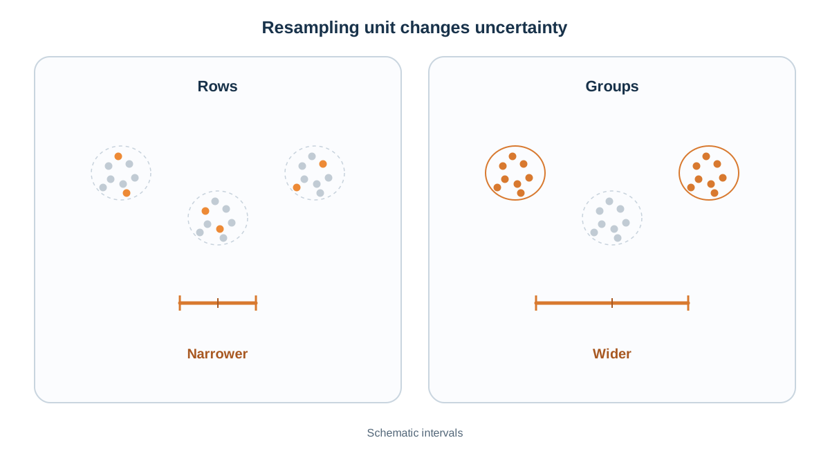
Grouped data. If rows come in clusters — multiple measurements per patient, multiple sessions per user, multiple rows per store — resampling rows breaks the dependence. The bootstrap treats correlated observations as fresh information, so the interval comes out narrower than it should. The fix is to resample whole groups, not rows.

Time-ordered data. Same trap with a direction. Resampling rows shuffles the future into the past and produces an interval describing a world where time does not exist. Use a block or moving-window scheme instead.

A biased sample cannot be rescued. The bootstrap resamples your sample. If the sample is wrong, the interval is a precise statement about the wrong thing. Precision is not accuracy.

Small n and tail statistics. With very few observations, the empirical distribution is a poor stand-in for the population. For statistics driven by the tails — maxima, rare quantiles — the bootstrap is unreliable regardless of how many replicates you draw.

Common mistake: Cranking B from 1,000 to 100,000 to "make the interval more accurate." More replicates reduce Monte Carlo noise in your estimate of the interval; they do nothing about a wrong resampling unit or a biased sample. Fix the unit first.

Before you run anything, apply this decision rule: name the unit, name the dependence, and ask whether a random resample of those units could plausibly have been produced by the real data-generating process. If not, resample at the group or block level instead.

Modify the Experiment: Change the Statistic and the Unit

One variation turns a copied script into a reusable pattern.

First, swap the mean for the median and compare:

median_replicates = bootstrap_replicates(data, np.median, B, rng)
print(f"Median 95% interval: "
      f"{np.quantile(median_replicates, [0.025, 0.975])}")

The median's interval is typically wider and its distribution more skewed. That is a concrete demonstration that uncertainty is a property of the statistic, not just the data.

Now break it on purpose. Build a small grouped dataset where each group contributes several correlated rows, then run two bootstraps on the same data: one that resamples rows and one that resamples whole groups.

# 40 groups, 5 correlated rows each. Group effect dominates.
n_groups, rows_per_group = 40, 5
group_effect = rng.normal(0, 3.0, size=n_groups)
rows = group_effect.repeat(rows_per_group) + rng.normal(0, 0.5,
                                                       size=n_groups * rows_per_group)
group_ids = np.repeat(np.arange(n_groups), rows_per_group)

def bootstrap_rows(x, stat, B, rng):
    n = len(x)
    return np.array([stat(rng.choice(x, size=n, replace=True)) for _ in range(B)])

def bootstrap_groups(x, groups, stat, B, rng):
    unique = np.unique(groups)
    out = []
    for _ in range(B):
        picked = rng.choice(unique, size=len(unique), replace=True)
        sample = np.concatenate([x[groups == g] for g in picked])
        out.append(stat(sample))
    return np.array(out)

row_reps = bootstrap_rows(rows, statistic, B, rng)
grp_reps = bootstrap_groups(rows, group_ids, statistic, B, rng)

print("Row-resampled 95% interval:",
      np.quantile(row_reps, [0.025, 0.975]))
print("Group-resampled 95% interval:",
      np.quantile(grp_reps, [0.025, 0.975]))

The row-resampled interval will be noticeably narrower. The group-resampled interval is wider because it accounts for the fact that rows within a group are not independent pieces of evidence. The gap between the two intervals is the cost of ignoring dependence. Keep the seed fixed across both runs so the only thing that changed is the resampling unit — that is what makes the comparison an experiment instead of an anecdote.

This is an illustrative construction, not a claim about any real dataset. The point is the mechanism: when the unit changes, the interval changes, and the narrower one is the one lying to you.

Record five fields alongside every result: the seed, the statistic, B, the confidence level, and the resampling unit. Without all five, the number is not reproducible and not comparable to the next run.

Make It a Habit

Before you report any estimate, run the bootstrap, look at the distribution, and write down the resampling unit. The distribution is the evidence; the interval is just a summary of it.

Your next step: take one number you currently report without an interval — a conversion rate, a mean latency, a model score — and run this exact loop on it. Then ask whether the interval is narrow enough to support the decision you are making with it. If the answer is no, you have learned something more useful than the number itself.

When the unit turns out not to be a single row, the natural follow-up is dependence-aware validation: grouped and time-based resampling schemes that match the structure of your data instead of pretending it is flat.