
How Bootstrap Resampling Builds an Interval for a Statistic
You have a thousand bootstrap replicates sitting in a NumPy array. You have a histogram. What you do not have is the two numbers you actually need to…

Key topics
You have a thousand bootstrap replicates sitting in a NumPy array. You have a histogram. What you do not have is the two numbers you actually need to report.
That gap is where most beginners stall. The replicates are easy to generate; the interval is where the thinking starts. And the first instinct — "the interval is just the middle 95% of the replicates" — is a real method with a real name. It is also only one of several ways to read the same pile of numbers, and the alternatives can disagree with it in ways that matter.
This article is about the mechanism that turns replicates into an interval, why two reasonable methods produce different endpoints from identical data, and what has to be true about your data for either interval to mean anything.
From Replicates to an Interval: What the Bootstrap Distribution Approximates
Before any formula, fix the notation. It will keep the rest of the article honest.
- θ (theta) is the true parameter you care about — the population standard deviation, the population median, whatever the statistic estimates. You never observe it.
- θ̂ (theta-hat) is your estimate computed from the one sample you actually have.
- θ̂* (theta-hat-star) is a bootstrap replicate: the same statistic computed on a resample drawn with replacement from your original sample.
- The bootstrap distribution is the collection of all your θ̂* values — the histogram you already have.
Two distributions are in play, and confusing them is the root of most interval confusion.
The sampling distribution of θ̂ describes how your estimate would vary if you drew many fresh samples from the population. It is centered near θ, and its spread is the uncertainty you want to quantify. You cannot see it, because you only get one sample.
The bootstrap distribution of θ̂* describes how your estimate varies when you resample from your sample. It is centered near θ̂, and you can see it completely.
The bootstrap principle is a single substitution: treat the pair (θ̂*, θ̂) as a stand-in for the pair (θ̂, θ). The empirical distribution of your sample plays the role of the unknown population distribution. If that substitution is reasonable, the spread of the bootstrap distribution approximates the spread of the sampling distribution, and you can read uncertainty off the replicates.
Every interval method below is a different way of exploiting that one substitution. They differ in which function of (θ̂*, θ̂) they use to approximate the corresponding function of (θ̂, θ).
Note: The substitution is asymptotic in spirit. It leans on the empirical distribution being a decent proxy for the population — a claim about sample size and about how the data were drawn. Small samples and non-representative samples weaken it.
Knowledge check
Check your understanding
Answer this question before you continue.
The Percentile Interval: Read the Quantiles Directly
The percentile interval is the most direct reading of the bootstrap distribution. Sort your replicates, take the α/2 and 1−α/2 quantiles, and report them. For a 95% interval, that is the 2.5th and 97.5th percentiles of the sorted θ̂* values.
The logic is causal and simple. If the bootstrap distribution approximates the sampling distribution, then the spread of replicates approximates the spread of the estimate, so the quantiles of the replicates approximate the quantiles of the estimate's uncertainty.
One property makes this method attractive: it is transformation invariant. If you apply a monotone transformation to your statistic — say you work with log-relative-risk instead of relative risk — the percentile interval for the transformed statistic is just the transformation of the percentile interval for the original. Two people working on different scales get equivalent answers. That is not true of every method.
The failure direction is worth naming. The percentile interval is asymmetric in whatever direction the bootstrap distribution is skewed. When the sampling distribution is biased or strongly skewed, the percentile interval can be asymmetric in the wrong direction, or not asymmetric enough. It has no clean derivation from a pivot, which is exactly why it is intuitive and also why mature tooling does not default to it.
Knowledge check
Check your understanding
Answer this question before you continue.
The Basic Interval: Mirror the Replicates Around the Estimate
The basic interval — also called the reverse percentile interval — starts from a pivot argument instead of a direct reading.
Approximate the distribution of θ̂ − θ by the distribution of θ̂* − θ̂. Then invert that approximation to get limits for θ. The derivation is short. Let q_low be the α/2 quantile of the bootstrap replicates θ̂*, and q_high the 1−α/2 quantile. The percentile interval is simply [q_low, q_high]. The basic interval reflects those same quantiles around the estimate:
In words: the lower limit is twice the estimate minus the upper bootstrap quantile, and the upper limit is twice the estimate minus the lower bootstrap quantile. The interval is the mirror image of the percentile interval around θ̂.
Make the geometry concrete. The basic interval reaches as far above θ̂ as the percentile interval reaches below it. The two intervals are reflections of each other around the estimate.
That mirror helps under simple bias and hurts under skewness. When the bootstrap distribution is skewed, the basic interval moves in the direction a naive reader does not expect — it does exactly the wrong thing. The tradeoff is plain: the basic interval has a clearer derivation and worse behavior on skewed statistics; the percentile interval has no derivation and better behavior on skewed statistics. Neither dominates.
Knowledge check
Check your understanding
Answer this question before you continue.
A Worked Example: Same Replicates, Two Different Intervals
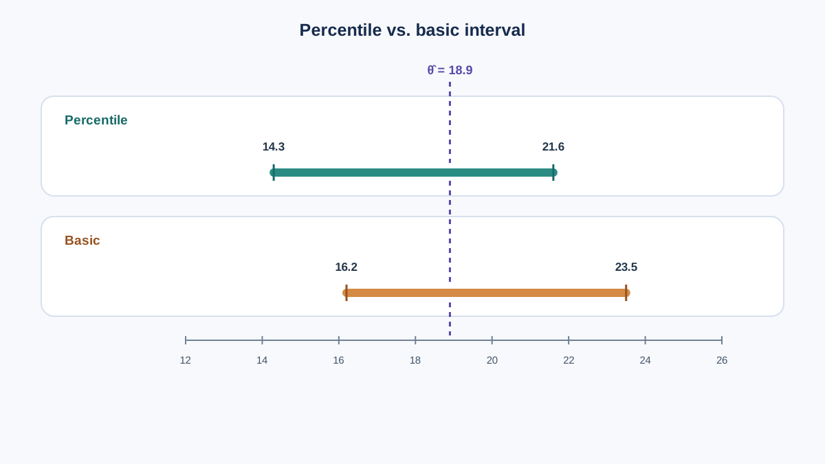
Numbers make the disagreement visible. Suppose you have eight observations of weekly hours worked, and you want an interval for the population standard deviation. The sample is skewed — a few zeros pull the distribution left — so the bootstrap distribution of the standard deviation will be asymmetric.
Say your point estimate is θ̂ = 18.9, and from 500 bootstrap replicates you extract these quantiles for a 90% interval:
- 5th percentile of θ̂*: 14.3
- 95th percentile of θ̂*: 21.6
The percentile interval is read straight off:
The basic interval mirrors those quantiles around the estimate:
| Method | Lower | Upper | Width |
|---|---|---|---|
| Percentile | 14.3 | 21.6 | 7.3 |
| Basic | 16.2 | 23.5 | 7.3 |
Same replicates. Same width. Different location. The basic interval sits higher because the bootstrap distribution is skewed left: the short tail below θ̂ gets mirrored into a short reach above it, and the long tail above gets mirrored into a long reach below. Under skewness, the mirror moves the interval in the direction opposite to what the percentile method does.
The practical consequence: the choice of method changes the reported uncertainty. That choice belongs in your experiment record, not in an unstated default. And the number of resamples controls the resolution of the quantile estimates — with only 500 replicates, the 5th and 95th percentiles are themselves noisy, so the endpoints carry resampling noise on top of sampling noise.
Common mistake: Treating the two intervals as interchangeable because they come from the same replicates. They come from the same replicates and answer slightly different questions about where θ sits.
Assumptions That Decide Whether the Interval Means Anything
The whole procedure rests on conditions. When one fails, the interval stops meaning what you think it means.
The resampling unit must match the dependence structure. Independent observations can be resampled individually. Grouped, clustered, or time-ordered data need a resampling scheme that preserves that structure — resample whole groups, or resample blocks in time order. Resampling individual rows from grouped data destroys the dependence and produces intervals that are too narrow.
The empirical distribution must be a reasonable stand-in for the population. This is a statement about sample size and about whether the sample was drawn in a way that represents the target population. A biased sample produces a biased bootstrap distribution, and no amount of resampling fixes it.
The statistic should not be wildly non-smooth or dominated by a few extreme observations. When it is, the bootstrap distribution is unstable and the quantiles move around between runs. If your endpoints jump when you change the random seed, that instability is the signal.
Coverage is approximate, not guaranteed. The interval is a statement about the sampling variability of the estimate under the assumed resampling scheme. It is not a promise that θ falls inside it with exactly the nominal probability.
The interval describes uncertainty in the estimate — not the spread of individual observations, and not the model's predictive performance. Conflating those three is the most common misreading. A bootstrap confidence interval for a mean is not a prediction interval for the next observation.
Knowledge check
Check your understanding
Answer this question before you continue.
Choosing a Method and Reporting It Honestly
Here is the decision rule I would apply.
Start with the percentile interval when the statistic is skewed or the sample is small — it handles asymmetry in the right direction. Use the basic interval when you want the pivot-based derivation and the statistic is roughly symmetric. Treat both as approximations, not final answers.
That heuristic has a boundary. Neither percentile nor basic is a universal choice, and the preference above is a starting point, not a guarantee. The right move is to check method sensitivity: compute both endpoints from the same replicates and see how far apart they land. When skewness or bias is consequential — when the interval drives a decision — escalate to bias-corrected and accelerated (BCa) methods. They exist precisely because percentile and basic intervals misbehave in those regimes, and they are the practical default in mature tooling.
Whatever you choose, record it. An interval without the statistic, the resampling unit, the number of resamples, the confidence level, and the method is not reproducible. Someone reading your result six months later needs all five.
And keep the boundary clear: an interval on a statistic is a different object from a validation estimate of generalization. Do not swap them in a report. One quantifies the variability of an estimate under stated assumptions; the other estimates how a model will perform on unseen data. They answer different questions.
The honest limit is this: bootstrap intervals are a tool for quantifying variability under stated assumptions, and the assumptions are the part that deserves the most scrutiny.
Run both methods on your own statistic. Compute the percentile and basic endpoints from the same replicates, put them side by side, and look at where they diverge. That divergence is not a bug — it is the shape of your bootstrap distribution telling you which assumption is doing the work.
Knowledge check
Final check
Finish the article by checking the ideas you just learned.
References
Build stronger machine learning foundations
Use structured resources to connect theory, scikit-learn workflows, and evaluation practice.


