
Batch Inference With Scikit-Learn: Turn a Saved Model Into Repeatable Predictions
You trained a model. You saved it. Now a new file of rows arrives, and each one needs a prediction. This is where a saved model proves its worth—or quietly…

Key topics
You trained a model. You saved it. Now a new file of rows arrives, and each one needs a prediction. This is where a saved model proves its worth—or quietly fails.
Here is the tension: a saved model is not a magic oracle. It is a frozen recipe. It only works if the new data arrives in the exact shape the model learned to consume. Get the shape right, and predictions flow out row by row. Get it wrong, and the model may still produce numbers—just numbers that mean nothing, with no error to warn you.
Batch inference in scikit-learn is the discipline of turning a saved artifact into repeatable predictions. Let's walk through what that actually involves.
What Batch Inference Actually Is
Batch inference means running a fitted model over a set of new rows at once, producing one prediction per row. Instead of asking the model about a single customer or a single house, you hand it a whole file or table and let it work through every row in one pass.
Three things are true at inference time that were not true during training:
The model is frozen. No fitting happens. The learned parameters and preprocessing steps are reused exactly as they were saved. The model does not adapt to the new data; it applies what it already learned.
The rows have no known answer. During training, every row had a target value the model could learn from. During evaluation, you compared predictions against known labels to measure quality. During inference, you are applying the model to rows where the answer is unknown. That is the whole point: you want the model to tell you something you do not already know.
The work happens in batches, not one request at a time. This distinguishes batch inference from real-time inference, where a single row arrives and needs an immediate prediction behind an API. Batch inference is the file-and-table version: process everything together, write the results somewhere durable, and move on.
A simple flow looks like this:
Saved pipeline (model + preprocessing) → New data file → Predictions
The training run ended before this flow started. Everything from here forward is inference.
Knowledge check
Check your understanding
Answer this question before you continue.
Why Preprocessing Must Travel With the Model
If you have worked with scikit-learn pipelines, you already know the core rule: the thing you save is not just the estimator. It is the whole preprocessing workflow—the scaler that standardized your features, the encoder that handled categorical columns, the imputer that filled missing values—bundled together with the model.
That bundling is not a convenience. It is a survival requirement.
Here is why. Imagine you trained a model on scaled features, where every numeric column was transformed to have a mean near zero and a standard deviation near one. The model learned its decision boundaries in that scaled space. Now you load the saved model and feed it raw, unscaled numbers. The values are ten times larger than anything the model saw. The predictions come back silently wrong. No error. No warning. Just confident nonsense.
The same failure happens with categorical data. If your training pipeline one-hot encoded a categorical column into several binary columns, the model expects that expanded shape. Feed it the original text column, and the model either crashes on a shape mismatch or—worse—interprets the data as something it was never trained to understand.
The pipeline object is the safe container because it removes the possibility of forgetting. When you call predict on a pipeline, it runs the transforms and then the model in one step. The preprocessing cannot be skipped because it is built into the path.
One distinction matters here: preprocessing at inference time is transform-only, never fit. The scaler's mean and variance were learned during training. The encoder's category list was learned during training. At inference time, those steps only apply what they already know. They do not recalculate anything from the new data.
Knowledge check
Check your understanding
Answer this question before you continue.
Preparing New Data for Prediction
Before you call predict, the new data must satisfy a few conditions. Think of this as checking the model's ID requirements before letting it through the door.
Same feature columns, same order, same names. The new data must contain the same feature columns the model was trained on. If the model was trained on price, sqft, and location, your new file needs those three columns—not cost instead of price, and not sqft in a different position. Scikit-learn's feature_names_in_ attribute can help you verify alignment when your pipeline was fitted on a DataFrame with named columns.
No target column. The new rows do not have the answer column, because you are asking the model to produce it. If your training file had a price column that was the target, your new file should not include it.
Extra columns must be handled deliberately. Real files often carry an ID column—a customer number, an application ID, a row identifier. That column is not a feature. The model never saw it during training, and it must be dropped before prediction. But do not throw it away entirely. You will need it later to attach predictions back to their rows.
Missing values follow the training rules. If your pipeline includes an imputer, it will handle missing values in the new data the same way it did during training. If it does not, missing values will cause an error. Either way, you cannot silently introduce a column the model never saw.
The practical loading step looks like this: read the CSV into a DataFrame, select the feature columns, and confirm the shape matches what the model expects. If the model expects twelve features and your DataFrame has twelve columns, you are ready. If it has thirteen, you probably left the ID column in.
Note: A successful
predictcall proves compatibility, not correctness. Three different things can happen when you feed new data to a saved model. The input can be rejected with an error. The input can be accepted but semantically wrong—right number of columns, wrong meaning. Or the input can be correct, and the model still makes an inaccurate prediction because no model is perfect. Only the first case announces itself. The other two require you to check your work.
Knowledge check
Check your understanding
Answer this question before you continue.
What Comes Out of predict
The output of predict is deceptively simple: an array with one entry per input row, in the same order as the input.
For regression, each entry is a numeric value—a predicted price, a predicted score, a predicted quantity.
For classification, each entry is a predicted class label—"approved" or "denied," "spam" or "not spam."
If you want more than a hard label, predict_proba is the companion method. It returns the probability the model assigns to each class. This matters when a downstream decision rule needs more than a yes-or-no answer. A loan model might label an application "approved," and the probability behind that label—0.51 versus 0.97—can change how you act on it. But treat those probabilities as model outputs, not guarantees of real-world certainty. Their usefulness depends on how the classifier was trained and assessed.
The critical property of the output is its order. Prediction number zero corresponds to input row zero. Prediction number one corresponds to input row one. That order is the foundation for attaching predictions back to the original data.
Input rows (with IDs) → predict() → Prediction array (same order)
But order is only trustworthy if nothing shuffled, dropped, or reordered the rows along the way.
Keeping Row Identity Straight
Here is the mistake I see beginners make most often: they run predictions, get an array of numbers, and then try to figure out which prediction belongs to which row by counting positions.
That works only if you can guarantee the rows never changed order. The moment you drop rows with missing values, filter the data, or shuffle it, the positional mapping breaks. Your prediction array no longer lines up with your original file, and you have a silent data disaster: predictions attached to the wrong customers, with no error to tell you.
The safest pattern is to keep the prediction input frame intact and attach predictions to it directly:
- Load the new data.
- Separate the ID column from the feature columns.
- Keep the feature rows in the same order you loaded them.
- Call
predicton those rows. - Attach the prediction array to the scored frame that still holds the IDs.
If you instead drop rows before predicting, or filter the data, then attach predictions later by joining on an ID, you must validate that join. An ID-based join is only safe when the ID is unique, was retained through every filtering step, and matches exactly the rows that were scored. Duplicate or stale IDs can produce a wrong join that looks perfectly orderly.
The difference comes down to two habits. Same-order assignment is simple and safe when you never drop or reorder rows. ID-based joining is more flexible but requires you to confirm the IDs are unique and aligned with the scored rows. Both beat guessing by position.
If you need to know which prediction belongs to which customer, preserve an ID column and keep it attached to the rows you actually scored. This is the difference between a script that works once on a clean file and a workflow you can trust on real data.
Knowledge check
Check your understanding
Answer this question before you continue.
Making Inference Repeatable
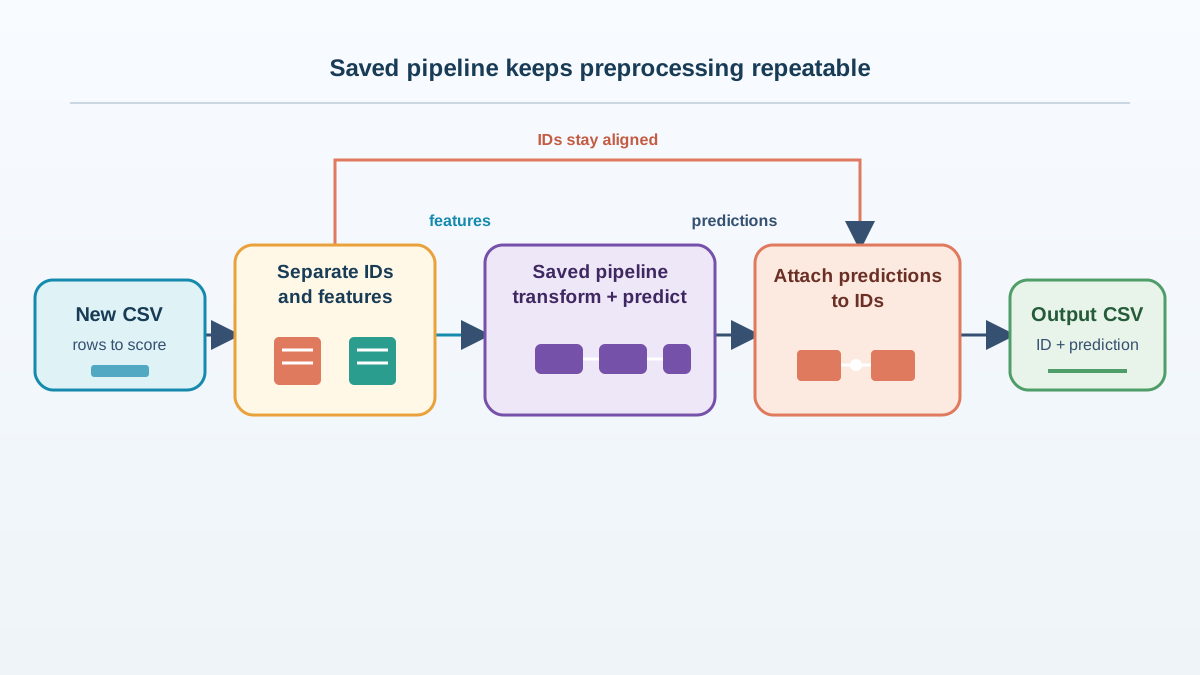
Repeatability means the same input file always produces the same predictions. That requires three things to stay fixed: the saved artifact, the preprocessing, and the absence of randomness at inference time.
A reusable inference script has a clear contract:
- Load the saved pipeline.
- Load the new data.
- Separate the feature columns from the ID column.
- Call
predicton the pipeline. - Write the predictions to an output file, paired with their IDs.
Loading the model once and reusing it across all rows is more efficient than reloading per row. Batch processing is naturally suited to this: one load, one transform, one prediction pass, one output file.
The output should be saved—to CSV, for example—so the predictions become a durable artifact others can inspect. A printed array in a notebook is not a deliverable. A file with IDs and predictions is.
Here is the boundary worth remembering: repeatability is not retraining. If you want better predictions, you do not tweak the inference script. You go back to training, improve the model, save a new artifact, and point your inference script at the new file. The script stays the same; the artifact changes. Keeping those two activities separate is what makes each one reliable.
Common Mistakes and How to Recover
Let's collect the failure modes so you can recognize them when they appear.
| Contract component | What breaks | How to recover |
|---|---|---|
| Saved artifact | Version mismatch between the scikit-learn version that saved the model and the one loading it | Check versions when loading; recreate the original environment if compatibility errors appear |
| Feature schema | Target column or ID column left in the input; wrong column names or order | Compare the input columns against feature_names_in_; drop anything that is not a feature |
| Preprocessing | Raw data fed to a model that expects scaled or encoded features | Use the pipeline object, which bundles transform and predict together |
| Row identity | Filtering or shuffling rows before prediction breaks the positional mapping | Keep an ID column attached to the scored rows; validate any ID-based join |
| Output | Predictions written without IDs, or attached to the wrong rows | Write the prediction array alongside the IDs from the exact rows that were scored |
The recovery pattern for all of these is the same: verify the loaded artifact on a small sample before running the full batch.
Take a few rows from your original training data, run them through the loaded pipeline, and confirm the predictions match what the saved workflow produced before. This is a smoke test: it catches loading errors, preprocessing mismatches, and version problems while they are still cheap to fix.
If you have rows with known answers, you can go one step further and compare predictions against those labels. But be careful about what you are testing. Expecting predictions to exactly match known labels is usually wrong—models make errors. If you want to measure prediction quality against known answers, use an appropriate evaluation metric, not a casual eyeball check. And remember: labels are not required for ordinary batch inference. Most real inference runs on rows where no one knows the answer yet.
Your Next Step
Write a small reusable inference script. It does not need to be elegant. It needs to do five things: load the saved pipeline, read a new CSV, separate the feature columns from the ID column, predict, and write the results to an output file with the ID column intact.
Then test it on a sample you already understand before you trust it on the full batch.
Inference is where a model earns its keep. Training built the capability; inference puts it to work. The discipline of keeping preprocessing intact, row identity preserved, and the workflow repeatable is what separates a model that works once from one that works every time.
Knowledge check
Final check
Finish the article by checking the ideas you just learned.
References
Research updated Sep 8, 2026

