
Why the Mean, Median, or Class Prevalence Is the Best Constant Baseline
You build a baseline, get a number, and have no idea whether that number is the best a constant can do or just a habit copied from a tutorial. Here is the…

Key topics
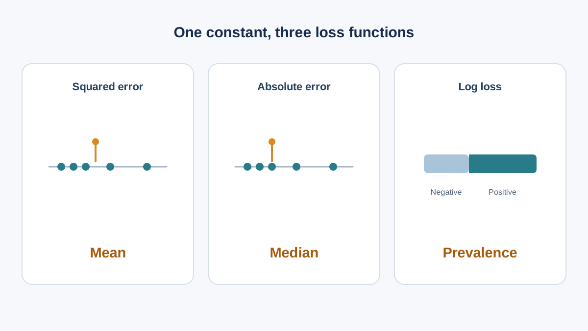
You build a baseline, get a number, and have no idea whether that number is the best a constant can do or just a habit copied from a tutorial. Here is the uncomfortable part: the mean, the median, and the class prevalence are not conventions. Each one is the closed-form solution to a specific loss function. Change the loss, and the "obvious" constant changes with it.
This article derives all three results from scratch, then turns each derivation into a baseline decision rule you can actually use.
The Constant Predictor as an Optimization Problem
A constant predictor is a model with no feature dependence. It ignores the input and outputs one value for every example. For regression, that value is a real number. For binary classification, it is a probability.
Let the training sample be . We want to choose a single scalar that minimizes the empirical risk:
Here is the loss function — the penalty for predicting when the truth is . We will minimize three of them: squared error, absolute error, and binary log loss.
The structural fact that makes this tractable: because the predictor is constant, the optimization collapses to a one-dimensional problem in a single scalar. That is why closed-form solutions exist. A model with features has one parameter per feature; a constant model has one parameter, period.
Three assumptions are baked in, and they matter:
- The sample is the object being optimized over. We are finding the best constant for this data, not for the population it came from.
- The loss is the one we declare. A different loss gives a different answer.
- The result is optimal for that sample and that loss — nothing more.
Note: A baseline must be evaluated under the same loss and the same split as the model it competes with. If you score your baseline with a different metric than your model, the comparison is meaningless.
If you need a refresher on constructing baselines and comparing them under a shared evaluation design, that groundwork is assumed here. This article is about why the constant takes the form it does.
Knowledge check
Check your understanding
Answer this question before you continue.
Why the Mean Minimizes Squared Error
Start with squared error. The loss for one prediction is , so the empirical risk is:
This is a smooth, convex function of . Differentiate with respect to :
Set the derivative to zero:
Divide both sides by and split the sum:
Since is constant, :
The optimal constant is the sample mean. The second derivative is , so this stationary point is the unique minimum. Convexity means there are no local-minimum traps — the mean is the global answer.
Interpretation: the mean is the point of balance. The minimized squared error equals the sample variance, which is why a constant model under MSE absorbs exactly the spread of the data and nothing else.
The failure mode follows directly from the mechanism. Squared error weights large deviations quadratically. A single extreme value drags the mean toward it and inflates the baseline error. This is not a separate rule to memorize — it is what the squared term does.
Connect to practice: when your evaluation metric is RMSE or MSE, the mean is the correct constant baseline. Reporting it tells you how much error a featureless model already absorbs.
Knowledge check
Check your understanding
Answer this question before you continue.
Why the Median Minimizes Absolute Error
Now switch to absolute error. The loss is , and the empirical risk is:
This function is piecewise linear with kinks at each data value . It is not differentiable everywhere, so the derivative argument from the previous section breaks down. We need a different tool.
Use the slope-counting argument. For a candidate value that sits between two data points, the slope of depends on how many points lie to the left versus the right. Each point to the left contributes a slope of ; each point to the right contributes . If points are below and are above, the slope is:
The minimum sits where this slope crosses zero — that is, where . The counts balance when half the data lies on each side. That point is a median.
But the slope argument only covers regions between data points. At a data value , the function has a kink, and the derivative does not exist. To handle that case, use the one-sided slopes. Just to the left of , the slope is , where counts points strictly below . Just to the right, it is , where counts points at or below . A minimum occurs at when the slope is non-positive on the left and non-negative on the right — that is, when neither side holds more than half the observations:
This condition defines the full set of medians. When is odd, exactly one data value satisfies it. When is even, an entire interval between the two middle values satisfies it, and every point in that interval is a minimizer. The minimizer is non-unique, and that is a real property of the objective, not a numerical artifact. Repeated values only widen the set of points that satisfy the condition.
The result generalizes. The -quantile minimizes the tilted absolute (pinball) loss, with the median as the special case. When over- and under-prediction cost different amounts, the optimal constant shifts toward a quantile other than the median.
Failure mode: absolute error is robust to outliers, but its objective is flat or kinked. That is why it is harder to optimize with gradient methods and why the minimizer can be non-unique.
Connect to practice: when your metric is MAE, the median is the correct constant baseline. The gap between the mean-baseline error and the median-baseline error is a quick diagnostic for how much outliers are distorting your target.
Knowledge check
Check your understanding
Answer this question before you continue.
Why Class Prevalence Minimizes Binary Log Loss
Classification is where learners most often get confused, because the predicted probability and the predicted label are two different decisions.
Define a constant probabilistic classifier: it outputs one probability for every input. Let be the number of positive examples and the number of negatives, with . Binary log loss is the average negative log-likelihood of the observed labels:
Differentiate with respect to :
Set to zero:
Cross-multiply and solve:
The optimal constant probability is the observed positive rate — the class prevalence. It is the same value regardless of which class you call positive.
Now separate two decisions that beginners conflate. The optimal constant probability is prevalence. The optimal constant hard label depends on the decision threshold and the cost of each error type. These are not the same question, and answering one does not answer the other.
There is a calibration connection worth noting, but it is narrower than it first appears. When prevalence is computed on the same sample you are optimizing over, the constant predictor is calibrated on that sample — its predicted probability matches the observed frequency by construction. That is an in-sample property. It does not guarantee calibration on a separate validation set or on future data, where the true positive rate may differ. Treat it as a reference point for checking whether a model's probabilities are trustworthy, not as a promise that survives the split.
Failure mode: with imbalanced classes, prevalence is a small number. Log loss rewards a confident-looking but nearly useless predictor. Always pair the log-loss baseline with a threshold-dependent metric such as accuracy, precision, or recall.
Connect to practice: when your metric is log loss or cross-entropy, the prevalence baseline is the number to compare against. The gap to a real model measures how much signal the features actually carry.
Knowledge check
Check your understanding
Answer this question before you continue.
One Objective, Three Answers: A Comparison
| Loss function | Optimal constant | Metric that makes it the right baseline |
|---|---|---|
| Squared error | Sample mean | MSE, RMSE |
| Absolute error | Sample median | MAE |
| Binary log loss | Class prevalence | Log loss, cross-entropy |
| Tilted absolute (pinball) | -quantile | Quantile loss |
The unifying principle: each optimal constant is the summary statistic that its loss function is designed to be minimized by. The pairing is not arbitrary — it falls out of the derivation.
For asymmetric loss, the optimal constant shifts toward a quantile other than the median. The median is a special case of a more general rule, not the whole story.
One boundary to flag: these results are for a single constant. They say nothing about whether a model with features can do better. That is a separate empirical question answered by validation, not by this derivation.
Turning the Derivation Into a Baseline Decision
Here is the workflow I would use.
Pick the constant baseline that matches your evaluation metric, not the one that is easiest to compute. The derivation tells you which constant is optimal for which loss. Ignoring that pairing means you are not measuring what you think you are measuring.
Three mistakes I see repeatedly:
Computing the mean baseline and then evaluating with MAE. This makes the baseline look worse than it is and inflates the apparent value of your model. The mean is not the MAE minimizer. The median is.
Reporting only the constant baseline's score without the metric's scale. A log-loss of 0.4 means nothing without knowing the prevalence. A MAE of 12 means nothing without knowing the target's range.
Treating the constant baseline as a formality rather than a diagnostic. A large gap between baseline and model on a small dataset is often noise, not signal. The baseline is a measurement instrument, not a checkbox.
A practical check: compute all three constants on the same training split and compare their errors under the matching metrics. This shows you how much the loss choice changes the story.
Common mistake: Fitting the constant on the full dataset and then scoring it on the same data. The constant should be fit on training data and scored on validation data, consistent with the split discipline you use for any other model.
The constant baseline is a solved optimization problem. The mean, median, and prevalence are each the provably optimal constant for one specific loss. Knowing which one applies turns the baseline from a ritual into a measurement instrument.
Your next step: take a dataset you already have. Compute the mean, the median, and the class prevalence on the training split. Score each under its matching metric. Those three numbers are the reference your candidate model should be compared against under the same evaluation design. If your model barely clears them, that is not a failure — it is evidence that the features are carrying little signal, and it is worth more than a higher score you cannot explain.
Knowledge check
Final check
Finish the article by checking the ideas you just learned.
References
Build stronger machine learning foundations
Use structured resources to connect theory, scikit-learn workflows, and evaluation practice.


